Overview

Galaxy clustering and the role of systematics

The angular two-point correlation function \(w(\theta)\) and the angular power spectrum \(C_\ell\) of galaxy number counts are among the most powerful probes of the large-scale structure (LSS) of the Universe. Comparing these statistics with theoretical predictions constrains cosmological parameters such as the matter density \(\Omega_m\), the dark energy equation of state \(w\), and the growth rate of structure \(f\sigma_8\).

Modern photometric galaxy surveys — including the Euclid mission, the Dark Energy Spectroscopic Instrument (DESI), and the Vera Rubin Observatory LSST — image billions of galaxies across thousands of square degrees of sky. The sheer statistical power of these datasets makes observational systematics the dominant source of systematic uncertainty in galaxy clustering analyses.

Observational systematics arise because the probability of detecting a galaxy in a given pointing of the telescope depends not only on the true galaxy density, but also on survey conditions:

Seeing (atmospheric point-spread function width) — poor seeing smears sources and reduces completeness for faint objects.
Galactic extinction — dust in the Milky Way absorbs and reddens background light, suppressing galaxy counts close to the Galactic plane.
Sky background — scattered moonlight or airglow raises the photon-noise floor, limiting depth.
Star density — bright stars mask patches of sky and their diffraction spikes affect neighbouring sources.
Survey depth variation — integration time, airmass, and camera throughput vary across the focal plane and across epochs.

Each of these effects can introduce coherent, large-scale fluctuations in the observed galaxy number counts that mimic or mask the genuine clustering signal. The key insight is that these systematic effects are spatially correlated with observable template maps — HEALPix maps of seeing, extinction, etc. — that can be constructed independently of the galaxy catalog.

sys_mapping provides a unified framework for inferring and correcting observational systematic contamination in galaxy overdensity maps. Six decontamination methods are implemented :

OLS — ordinary least-squares linear regression of the overdensity on the template maps, following Ross et al. 2011 (MNRAS 417, 1350) and Ho et al. 2012 (ApJ 761, 14).
ElasticNet — \(\ell_1+\ell_2\)-regularised regression with cross-validated template selection, following Weaverdyck & Huterer 2021 (MNRAS 503, 5061).
ISD-1 / ISD-3 — iterative systematic decontamination using first- or third-order polynomial template deprojection, following Rodríguez-Monroy et al. 2025.
MCMC-add — full Bayesian posterior sampling for a purely additive contamination model, following Elsner, Leistedt & Peiris 2016 (MNRAS 456, 2095) and Berlfein et al. 2024 (MNRAS 531, 4954).
MCMC-comb — full Bayesian posterior sampling for the combined additive-plus-multiplicative model, following Berlfein et al. 2024 (MNRAS 531, 4954).

All methods share the same contamination model, template normalisation, noise debiasing, and two-point function correction infrastructure described below. A full bibliographic review with method comparisons is on the Bibliography page; the method-to-paper map is on the Methods Reference page.

Notation and conventions

The table below defines every symbol used throughout the documentation and the source code. All maps use the HEALPix pixelisation with equal-area pixels; the pixel index is denoted \(p\).

Symbol	Definition
\(p\)	HEALPix pixel index, \(p = 0, \ldots, N_{\rm pix}-1\).
\(N_{\rm pix}\)	Total number of HEALPix pixels, \(N_{\rm pix} = 12\,{\rm NSIDE}^2\).
\(N\)	Number of unmasked pixels used in the fit.
\(n_g(p)\)	Observed galaxy count in pixel \(p\).
\(n_r(p)\)	Random catalog count in pixel \(p\) (uniform, no systematics).
\(\bar{n}_g\)	Mean galaxy count per pixel, \(\bar{n}_g = \sum_p n_g(p)/N\).
\(\delta_g(p)\)	True galaxy overdensity, \(\delta_g = n_g/\bar{n}_g - 1\).
\(\hat{\delta}_g(p)\)	Observed (contaminated) galaxy overdensity (what we measure).
\(t_i(p)\)	Systematic template map \(i\), normalised to zero mean and unit variance over the unmasked footprint. Indexed \(i = 1, \ldots, n_s\).
\(n_s\)	Number of systematic templates.
\(a_i\)	Additive contamination amplitude for template \(i\). Dimensionless; typical values \(\|a_i\| \lesssim 0.2\).
\(b_i\)	Multiplicative contamination amplitude for template \(i\). Dimensionless; typical values \(\|b_i\| \lesssim 0.3\).
\(\sigma\)	Pixel-to-pixel standard deviation of the clean overdensity field (a nuisance parameter in the likelihood).
\(\gamma\)	Skewness parameter of the skew-normal likelihood (used with lognormal galaxy fields; \(\gamma=0\) recovers Gaussian).
\(w(\theta)\)	Angular two-point correlation function, a function of separation angle \(\theta\).
\(C_\ell\)	Angular power spectrum at multipole \(\ell\) (Fourier dual of \(w(\theta)\) on the sphere).
\(\hat{\Theta}\)	Maximum likelihood estimate (MLE) / posterior median of the parameter vector \(\boldsymbol\Theta = (a_1,\ldots,a_{n_s}, b_1,\ldots,b_{n_s}, \sigma)\).
\(V\)	PCA rotation matrix (eigenvectors of the template covariance matrix).
\(\tilde{a}_i^2\)	Noise-debiased squared additive amplitude (used for two-point correction).
\(w_{\rm add/comb}(p)\)	Per-pixel systematic weight applied to galaxies in pixel \(p\).

Note

Throughout the code, arrays indexed over all pixels have shape (n_pix,) where n_pix = 12 * nside**2. Arrays indexed over unmasked pixels have shape (n_good_pix,) and are obtained by boolean-indexing with a good_pix mask. Template arrays have shape (n_sys, n_pix) or (n_sys, n_good_pix).

The observed galaxy overdensity

The galaxy overdensity at pixel \(p\) is estimated from the galaxy and random catalogs as (Landy-Szalay estimator at the pixel level):

\[\hat{\delta}_g(p) = \frac{n_g(p)}{f_r\,n_r(p)} - 1\]

where \(f_r = \bar{n}_g / \bar{n}_r\) is the ratio of the mean galaxy count to the mean random count, chosen so that \(\langle\hat\delta_g\rangle = 0\) over the unmasked footprint. Pixels where \(n_r(p) = 0\) or the mask equals zero are excluded.

In sys_mapping this is computed by compute_overdensity().

Systematic template maps

A systematic template map \(t_i(p)\) is an external HEALPix map that traces an observational condition expected to correlate with galaxy detection efficiency. Examples include:

dust extinction \(E(B-V)\) from Schlegel, Finkbeiner & Davis 1998;
stellar number density from Gaia or 2MASS;
seeing FWHM, sky background, airmass from survey logs;
HI column density from 21 cm surveys.

Before fitting, each template is normalised to zero mean and unit standard deviation over the unmasked footprint:

\[t_i(p) \;\leftarrow\; \frac{t_i(p) - \mu_{t_i}}{\sigma_{t_i}}, \qquad \mu_{t_i} = \frac{1}{N}\sum_{p \in \text{mask}} t_i(p), \quad \sigma_{t_i}^2 = \frac{1}{N}\sum_{p \in \text{mask}} t_i(p)^2 - \mu_{t_i}^2.\]

This normalisation ensures that the amplitudes \(a_i\) and \(b_i\) are on the same scale and that their priors can be specified uniformly.

Template maps can be generated synthetically with generate_systematic_map() or loaded from external files (HEALPix FITS format).

Contamination model

Physical interpretation. An additive systematic biases the galaxy overdensity by an amount proportional to the template value — for example, dust extinction adds a spurious decrement to galaxy counts in regions of high extinction. A multiplicative systematic modulates the overall amplitude of the galaxy overdensity — for example, variable seeing changes the survey depth and therefore scales galaxy counts up or down by a position-dependent factor.

The combined forward model is defined as in Berlfein+2024 (Eq. 13):

\[\hat{\delta}_{g}(p) = \underbrace{\delta_{g}(p)\!\left(1 + \sum_{i=1}^{n_s} b_i\,t_i(p)\right)}_{\text{multiplicative term}} + \underbrace{\sum_{i=1}^{n_s} a_i\,t_i(p)}_{\text{additive term}}\]

Three nested models are available, obtained by constraining the parameters:

Additive (\(b_i = 0\) for all \(i\)):

\[\hat{\delta}_{g}(p) = \delta_{g}(p) + \sum_{i=1}^{n_s} a_i\,t_i(p)\]

The observed overdensity is the true overdensity plus a linear combination of templates. This is the correct model for e.g. stellar contamination that adds spurious overdensity rather than modulating the galaxy selection. Free parameters: \(\{a_i\}_{i=1}^{n_s}\) plus \(\sigma\). Total: \(n_s + 1\).

Multiplicative (\(b_i = a_i\) for all \(i\), Eq. 12):

\[\hat{\delta}_{g}(p) = \delta_{g}(p)\!\left(1 + \sum_{i=1}^{n_s} a_i\,t_i(p)\right)\]

The template modulates the amplitude of the true overdensity. This is the correct model for depth variations: a seeing map that scales galaxy completeness uniformly across the true density field. Free parameters: \(\{a_i\}_{i=1}^{n_s}\) plus \(\sigma\). Total: \(n_s + 1\).

Combined (free \(a_i, b_i\)):

\[\hat{\delta}_{g}(p) = \delta_{g}(p)\!\left(1 + \sum_{i=1}^{n_s} b_i\,t_i(p)\right) + \sum_{i=1}^{n_s} a_i\,t_i(p)\]

The most general first-order model. For small amplitudes \(|a_i|, |b_i| \ll 1\) the full product \((\delta_g + a{\cdot}t)(1+b{\cdot}t)\) agrees with this expression to second order in the amplitudes (the cross-term \((a{\cdot}t)(b{\cdot}t)\) is negligible for typical survey systematics where \(|a|, |b| \lesssim 0.2\)). Free parameters: \(\{a_i, b_i\}_{i=1}^{n_s}\) plus \(\sigma\). Total: \(2n_s + 1\).

The model can be inverted to recover the clean overdensity from the observed one:

\[\delta_g(p) = \frac{\hat{\delta}_g(p) - \sum_i a_i\,t_i(p)}{1 + \sum_i b_i\,t_i(p)}\]

This inversion requires \(1 + \sum_i b_i\,t_i(p) > 0\) in every pixel (the denominator must be positive for the model to be physically consistent).

Method-to-model mapping. All six decontamination methods share the same forward model and inversion formula above, but differ in which model variant they target and how they estimate the parameters:

Method	Model variant	Parameter estimation
OLS	Additive (\(b_i = 0\))	Ordinary least-squares regression of \(\hat{\delta}_g\) on \(\{t_i\}\): solve \(\mathbf{X}\,\mathbf{a} = \hat{\boldsymbol\delta}_g\) where \(X_{pi} = t_i(p)\). (`run_decontamination()`)
ElasticNet	Additive (\(b_i = 0\))	\(\ell_1+\ell_2\)-regularised regression; regularisation strength \(\alpha\) and mixing ratio are chosen by \(k\)-fold cross-validation. (`elasticnet_contamination_fit()`)
ISD-1	Additive–multiplicative hybrid	Iterative reweighted OLS: at each iteration, pixel weights \(w(p) = 1/(1 + \hat{\mathbf{a}}\cdot\mathbf{t}(p))\) are recomputed from the current estimate and the regression is refit on the weighted residuals. Polynomial order 1 (linear templates only). (`iterative_systematics_decontamination()`)
ISD-3	Additive–multiplicative hybrid	Same iterative reweighted OLS as ISD-1, but the template basis is expanded with polynomial cross-terms up to order 3 before each fit. (`iterative_systematics_decontamination()`)
MCMC-add	Additive (\(b_i = 0\))	Bayesian posterior sampling (emcee ensemble sampler) of the Gaussian or skew-normal likelihood with \(b_i = 0\) fixed. Provides full posterior over \(\{a_i, \sigma\}\). (`run_mcmc()`)
MCMC-comb	Combined (free \(a_i, b_i\))	Bayesian posterior sampling of the full combined-model likelihood. The template basis is first PCA-rotated to decouple the parameters. Provides full posterior over \(\{a_i, b_i, \sigma\}\). (`run_mcmc()`, `rotate_templates()`)

Note

Regression methods (OLS, ElasticNet, ISD) return point estimates only. Parameter uncertainty is available analytically for OLS (from the least-squares covariance matrix) but is not estimated for ElasticNet or ISD. MCMC methods return full posteriors, from which variances and credible intervals can be extracted.

Gaussian log-likelihood (Eq. 17)

Assuming the true galaxy overdensity \(\delta_g(p)\) is drawn independently from a Gaussian distribution \(\delta_g(p) \sim \mathcal{N}(0, \sigma^2)\) in each pixel, the likelihood of the parameter vector \(\boldsymbol\Theta = (a_1, \ldots, a_{n_s}, b_1, \ldots, b_{n_s}, \sigma)\) given the observed overdensity \(\hat{\delta}_g\) and templates \(t_i\) is:

\[p(\hat{\boldsymbol\delta}_g \mid \boldsymbol\Theta) = \prod_p \frac{1}{\sqrt{2\pi\sigma^2}\,|1 + \sum_i b_i t_i(p)|} \exp\!\left[-\frac{\delta_g(p)^2}{2\sigma^2}\right]\]

where \(\delta_g(p) = (\hat\delta_g(p) - \sum_i a_i t_i(p))/(1+\sum_i b_i t_i(p))\) is the clean overdensity (see above). It is the residual after subtracting the contamination.

The factor \(|1 + \sum_i b_i t_i(p)|\) in the denominator is the Jacobian of the change of variables from \(\hat{\delta}_g\) to \(\delta_g\): differentiating the forward model gives \(\partial\hat{\delta}_g / \partial\delta_g = 1 + \sum_i b_i t_i(p)\), and this factor must be included so that the total probability integrates to 1. For a purely additive model (\(b_i=0\)) the Jacobian is 1 and vanishes from the likelihood.

Taking the logarithm yields (Eq. 17):

\[\ln\mathcal{L} = -\frac{N}{2}\ln(2\pi\sigma^2) - \underbrace{\sum_p \ln\!\left|1 + \sum_i b_i\,t_i(p)\right|}_{\text{Jacobian term}} - \underbrace{\frac{1}{2\sigma^2}\sum_p \delta_g(p)^2}_{\text{residual term}}\]

The Jacobian term penalises parameter combinations that make the multiplicative factor very different from 1 (i.e. very large \(|b_i|\) values), preventing the model from arbitrarily rescaling the variance.

The likelihood is JIT-compiled via JAX (make_log_likelihood()) and traced once per (n_sys, model, use_skewed) combination; subsequent evaluations run at near-native speed on CPU (\(\approx 300\;\mu{\rm s}\) per call at \(N = 10\,000\)).

Skew-normal log-likelihood (Eq. 18)

For a lognormal galaxy field the true overdensity \(\delta_g = e^{G-\sigma_G^2/2}-1\) (where \(G\) is Gaussian) has a positively skewed distribution. When systematics are weak, the skewness of the recovered \(\delta_g\) is approximately preserved, and fitting a Gaussian likelihood introduces a small but systematic bias.

The skew-normal extension adds a log-CDF correction term to the Gaussian log-likelihood:

\[\ln\mathcal{L}_{\rm skew} = \ln\mathcal{L}_{\rm Gauss} + N\ln 2 + \sum_p \ln\Phi\!\left(\gamma\,\frac{\delta_g(p)}{\sigma}\right)\]

where:

\(\gamma > 0\) is the skewness shape parameter (a fitted nuisance parameter; typical values \(0 < \gamma \lesssim 3\) for lognormal fields with \(\sigma_G \approx 0.5\)).
\(\Phi(z) = \frac{1}{2}\bigl[1 + \mathrm{erf}(z/\sqrt{2})\bigr]\) is the standard-normal CDF.
The mean of the skew-normal is \(\xi = -\sigma\,\delta\,\sqrt{2/\pi}\) with \(\delta = \gamma/\sqrt{1+\gamma^2}\), which is subtracted internally so that \(\mathbb{E}[\delta_g] = 0\) is maintained.
\(\ln\Phi(z)\) is evaluated as jax.scipy.special.log_ndtr(z) for numerical stability (avoids large-magnitude cancellation at negative \(z\)).

Setting \(\gamma = 0\) recovers the Gaussian likelihood exactly.

Template PCA rotation (Appendix A)

When the systematic template maps \(t_i(p)\) are correlated with each other (e.g. seeing and depth are correlated because both depend on observing conditions), the likelihood parameters \((a_i, b_i)\) are partially degenerate — many combinations of amplitudes produce the same observed contaminated field. This makes the posterior multimodal or poorly conditioned, leading to slow MCMC convergence.

The solution is a Principal Component Analysis (PCA) rotation of the template basis before fitting. The template covariance matrix is:

\[C_{ij} = \frac{1}{N}\sum_p t_i(p)\,t_j(p) \equiv \frac{1}{N}\,\mathbf{T}\mathbf{T}^\top\]

where \(\mathbf{T}\) is the \(n_s \times N\) matrix of template values. The eigendecomposition \(C = V D V^\top\) (with \(V\) orthogonal and \(D\) diagonal) gives a rotation matrix that diagonalises the template covariance. Rotated templates are defined by:

\[t'_j(p) = \sum_i V_{ij}\,t_i(p), \qquad \text{i.e.} \quad \mathbf{T}' = V^\top \mathbf{T}\]

In the rotated basis, \(C' = V^\top C V = D\) is diagonal by construction, so the rotated templates are orthogonal (their cross-pixel inner products vanish). Each rotated amplitude \(a'_j\) (or \(b'_j\)) is then independently constrained.

After MCMC inference in the rotated basis, parameters are transformed back to the original template basis via:

\[a_i = \sum_j V_{ij}\,a'_j \equiv (V\,\mathbf{a}')_i, \qquad b_i = \sum_j V_{ij}\,b'_j \equiv (V\,\mathbf{b}')_i\]

The rotation and back-transformation are implemented in rotate_templates() and transform_params_from_rotated().

Noise debiasing (Eq. 21)

After MCMC, the posterior median \(\hat{a}_i\) is an estimate of the true amplitude \(a_i\). The squared MLE however satisfies:

\[\mathbb{E}[\hat{a}_i^2] = a_i^2 + \mathrm{Var}[\hat{a}_i]\]

because the expectation of a squared random variable always exceeds the square of its expectation by the variance. This means the raw squared estimate over-estimates the true squared amplitude by the sampling variance.

The debiased squared amplitude is (Eq. 21):

\[\tilde{a}_i^2 = \max\!\bigl(\hat{a}_i^2 - \mathrm{Var}[\hat{a}_i],\; 0\bigr)\]

and analogously for \(\tilde{b}_i^2\). The \(\max(\cdot, 0)\) clip is necessary because sampling noise can produce \(\hat{a}_i^2 < \mathrm{Var}[\hat{a}_i]\) (this happens when the true amplitude is small and the posterior variance is large). Clipping to zero enforces the physical constraint \(a_i^2 \geq 0\).

The variance \(\mathrm{Var}[\hat{a}_i]\) is estimated from the MCMC chain via get_param_variance_from_chain() as the posterior variance (the diagonal of the posterior covariance matrix).

Two-point function correction (Eq. 15–16)

The observed angular two-point correlation function \(\hat{w}(\theta)\) is related to the true galaxy two-point function \(w_g(\theta)\) by the contamination model. To first order in the amplitudes (assuming \(|a_i|, |b_i| \ll 1\)):

\[\hat{w}(\theta) \approx w_g(\theta)\!\left[1 + \sum_i b_i^2\,w_{t_i}(\theta)\right] + \sum_i a_i^2\,w_{t_i}(\theta)\]

where \(w_{t_i}(\theta) = \langle t_i(\hat{n})\,t_i(\hat{n}')\rangle_\theta\) is the angular auto-correlation of template \(i\) at separation \(\theta\). This expression is derived by inserting the contamination model into the definition of the two-point function and expanding to first order in \(a_i b_i\) (the cross-term is \(\mathcal{O}(a_i b_i)\) and is neglected).

Inverting for the true clustering:

\[\hat{w}_{\rm corr}(\theta) = \frac{\hat{w}(\theta) - \sum_i \tilde{a}_i^2\,w_{t_i}(\theta)} {1 + \sum_i \tilde{b}_i^2\,w_{t_i}(\theta)}\]

where the debiased amplitudes \(\tilde{a}_i^2, \tilde{b}_i^2\) (from debias_params()) are used to avoid noise amplification.

The template two-point functions \(w_{t_i}(\theta)\) are estimated from the template maps directly using the same estimator as for the galaxy field. The corrected \(\hat{w}_{\rm corr}(\theta)\) should be free of systematic bias to first order in the contamination amplitudes.

The correction is implemented in correct_two_point_function().

Model selection (Eq. 19)

To decide whether the data require the full combined model (both additive and multiplicative terms) or whether the simpler additive model is sufficient, we use the likelihood ratio test (LRT).

Given two nested models — a null model \(\mathcal{M}_0\) with parameter count \(k_0\) (e.g. additive with \(n_s + 1\) parameters) and an alternative model \(\mathcal{M}_1\) with \(k_1 > k_0\) parameters (e.g. combined with \(2n_s + 1\)) — the LRT statistic is:

\[\lambda_{\rm LR} = 2\!\left[\ln\mathcal{L}(\hat{\Theta}_1) - \ln\mathcal{L}(\hat{\Theta}_0)\right]\]

where \(\hat{\Theta}_0\) and \(\hat{\Theta}_1\) are the MLEs under each model. Under the null hypothesis (that \(\mathcal{M}_0\) is correct), Wilks’ theorem guarantees that:

\[\lambda_{\rm LR} \xrightarrow{N\to\infty} \chi^2(r), \qquad r = k_1 - k_0\]

For the additive vs combined comparison, \(r = n_s\) (the number of additional multiplicative parameters \(b_i\)).

The p-value is \(P(\chi^2(r) > \lambda_{\rm LR})\) from the chi-squared CDF. Typical decision threshold: reject \(\mathcal{M}_0\) at the 5 % significance level when \(\lambda_{\rm LR} > \chi^2_{r,\,0.95}\).

The LRT is implemented in likelihood_ratio_test().

Note

The asymptotic \(\chi^2\) approximation holds for large \(N\) (many unmasked pixels). At NSIDE = 64 with a Galactic cut there are \(\approx 32\,000\) unmasked pixels, which is more than sufficient for the approximation to be excellent.

Per-galaxy systematic weights

For catalog-level analyses (e.g. passing corrected galaxy positions to a two-point function estimator such as TreeCorr or Corrfunc), the contamination correction is encoded as a per-galaxy weight. Rather than modifying the galaxy catalog, each galaxy in pixel \(p\) receives a weight that effectively rescales its contribution to the clustering statistics.

The weight is derived from the MAP (Maximum A Posteriori) parameter estimates. The MAP estimate \(\hat{\Theta}\) is the mode of the posterior distribution \(p(\Theta \mid \text{data}) \propto \mathcal{L}(\text{data} \mid \Theta)\,p(\Theta)\); in practice it is approximated by the posterior median of the MCMC chain. For the non-Bayesian methods (OLS, ElasticNet, ISD) there is no explicit prior, so the MAP reduces to the maximum-likelihood estimate (MLE).

The corrected overdensity is:

\[\delta_g(p) = \frac{\hat{\delta}_g(p) - \sum_i \hat{a}_i\,t_i(p)}{1 + \sum_i \hat{b}_i\,t_i(p)}\]

Dividing by the number density, the natural weight for the additive correction is:

\[w_{\rm add}(p) = \frac{1}{\max\!\left(1 + \sum_i \hat{a}_i^{\rm add}\,t_i(p),\;\epsilon\right)}\]

where \(\hat{a}_i^{\rm add}\) are the MAP additive-model parameters. For the combined model, the multiplicative term modulates the selection function, so the appropriate weight uses the MAP multiplicative parameters:

\[w_{\rm comb}(p) = \frac{1}{\max\!\left(1 + \sum_i \hat{b}_i^{\rm comb}\,t_i(p),\;\epsilon\right)}\]

The clip \(\epsilon = 0.01\) prevents division by near-zero or negative denominators (which would correspond to unphysical negative weights). Galaxies in pixels with no valid template coverage receive \(w = 1\) (no correction).

In practice, scripts/compute_sys_weights.py writes three columns to the output FITS file:

WEIGHT_ADD — additive-model weight (using \(\hat{a}_i^{\rm add}\))
WEIGHT_COMB — combined-model weight (using \(\hat{b}_i^{\rm comb}\))
``WEIGHT_SYS`` — recommended default; identical to WEIGHT_COMB

The combined model is always superior to the additive-only model across all contamination regimes (see Model test matrix), so WEIGHT_SYS / WEIGHT_COMB should be used unless there is a specific reason to prefer the additive model (e.g. debugging or speed).

Summary of the workflow

The standard analysis pipeline proceeds as follows. Steps 1–2 and 4–7 are shared by all six methods; step 3 branches by method.

Load catalog and templates — pixelise galaxy and random catalogs into HEALPix maps; load and normalise template maps. (pixelize_catalog(), compute_overdensity(), assign_template_values())
Template selection and deduplication — rank templates by signal-to-noise of their cross-correlation with the overdensity; remove near-duplicates within each systematic family. (snr_template_ranking())
Parameter estimation — run one or more decontamination methods via the unified interface (run_decontamination()):
- OLS — ordinary least-squares fit of the additive model (seconds).
- ElasticNet — cross-validated regularised regression, additive model (seconds to minutes).
- ISD-1 / ISD-3 — iterative reweighted regression, additive–multiplicative hybrid (minutes).
- MCMC-add — Bayesian posterior sampling, additive model. The template basis is first PCA-rotated (rotate_templates()) to decouple parameters before sampling (hours).
- MCMC-comb — Bayesian posterior sampling, combined model; same PCA-rotation pre-processing (hours).
Model selection — compare model fits to choose between the additive and combined models. For MCMC methods: likelihood ratio test (likelihood_ratio_test()). For ElasticNet: cross-validation scores guide template and regularisation selection. For OLS / ISD: SNR-based template ranking suffices.
Noise debiasing — subtract the parameter variance from the squared MAP estimates to correct for the noise bias in the two-point correction. (debias_params())
Two-point correction — apply the debiased amplitudes to the measured \(\hat{w}(\theta)\) to recover the uncontaminated \(w(\theta)\). (correct_two_point_function())
Diagnostics — null tests, SNR ranking, footprint masking sensitivity. (diagnostics)

For a hands-on implementation of this pipeline see the Quickstart. For theoretical background on each step with full paper references see Methods Reference. For mock-catalog validation results see End-to-end validation.

Analysis execution pipeline

The mathematical pipeline above describes what happens inside a single bin for a single method. The orchestration layer decides the order in which datasets and methods are processed. This section describes that outer layer, which was designed to give researchers a fast preview of preliminary results without waiting for the slowest (MCMC) methods to complete.

Motivation — method-first execution

sys_mapping implements six decontamination methods that span several orders of magnitude in runtime. The table below gives measured wall-clock times per sample for the LS10 BGS analysis (11 templates, NSIDE 32–256):

Method	NSIDE 32 (≈ 5 600 pix)	NSIDE 64 (≈ 21 600 pix)	NSIDE 128 (≈ 84 600 pix)	When to use
OLS	< 0.01 s	< 0.01 s	< 0.12 s	Quick first-pass; linear regression closed-form solution
ISD-1	< 0.01 s	0.05–0.30 s	0.23–1.42 s	Iterative additive model; see Rodríguez-Monroy et al. 2025
ElasticNet	0.1–0.9 s	1–30 s	4–73 s	Automatic template selection via cross-validated regularisation
ISD-3	55–90 s	100–190 s	n/a	Degree-3 polynomial expansion; ill-conditioned with correlated templates
MCMC-add	~23 s	75–101 s	~5 min (est.)	Full Bayesian posterior for additive model
MCMC-comb	~31 s	~116 s	~7 min (est.)	Full Bayesian posterior for combined additive+multiplicative model

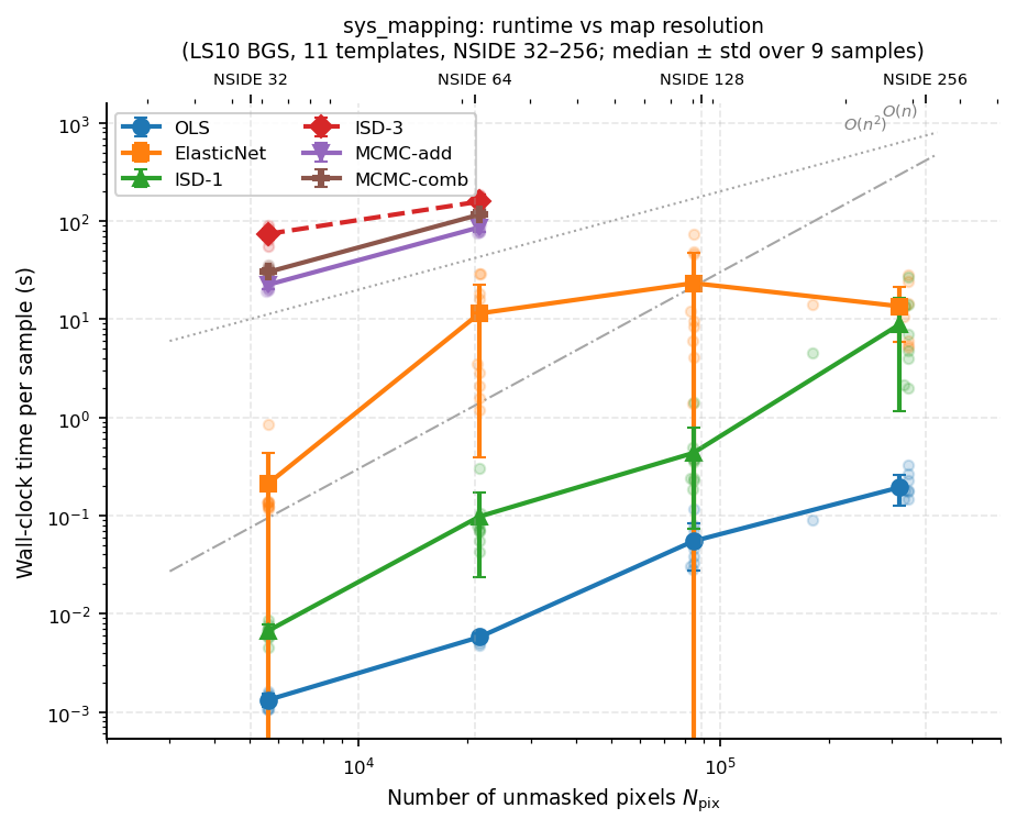
The figure below shows how each method’s runtime scales with the number of unmasked pixels, using all available LS10 BGS measurements (9 samples × 4 resolutions). OLS and ISD-1 scale as \(O(n)\), ElasticNet cross-validation is super-linear due to repeated fits, ISD-3 polynomial feature expansion is \(O(n^2)\) in practice, and MCMC scales linearly (each step evaluates the likelihood over all pixels).

Runtime vs n_pix for each decontamination method — Wall-clock time per sample vs number of unmasked HEALPix pixels for each decontamination method (LS10 BGS, 11 templates). Individual points (faint) show the 9 BGS VLIM samples; connected markers show the mean ± std per NSIDE. MCMC-add and MCMC-comb timings at NSIDE 32 are estimated by n\ :sub:`pix` scaling from NSIDE 64 measurements. Generated by ``scripts/plot_runtime_scaling.py``.

Rather than running all six methods inside a single run_bin() call (which forces the analyst to wait for the slowest MCMC method before seeing any results), the pipeline inverts the loop: method is the outer dimension, dataset/bin is the inner dimension. After the OLS phase finishes for all datasets, results are immediately written to the Sphinx documentation — the analyst can browse them in seconds. The MCMC phases then run in the background and progressively fill in the more precise estimates.

Execution phases

Phase 1 — OLS (< 1 s/dataset)
    LS10 BGS
    ↓ update docs/results_ls10.rst
    ↓ rebuild Sphinx HTML

Phase 2 — ElasticNet (seconds–minutes/dataset)
    ↓ update RST + rebuild HTML

Phase 3 — MCMC-add (1–2 min/dataset at NSIDE 64)
    ↓ update RST + rebuild HTML

Phase 4 — MCMC-comb (~2 min/dataset at NSIDE 64)
    ↓ full RST regeneration
    ↓ final Sphinx HTML rebuild

Dataset covered by the orchestrated run:

LS10 BGS — Legacy Survey DR10 Bright Galaxy Sample, NSIDE = 64, 11 observational templates (EBV, GALDEPTH_R, NOBS_R, PSFSIZE_R, and 7 Gaia photometry/star-density maps)

The orchestration script

The entry point is the bash script scripts/run_all_methods_sequential.sh. All behaviour is controlled through environment variables so the script itself never needs to be edited:

# Typical usage — nohup so the terminal can be closed
nohup bash scripts/run_all_methods_sequential.sh > logs/run_all.log 2>&1 &

# OLS-only quick preview (seconds)
METHODS="OLS" bash scripts/run_all_methods_sequential.sh

# Resume from MCMC-add (OLS and ElasticNet already done)
METHODS="MCMC-add MCMC-comb" bash scripts/run_all_methods_sequential.sh

# Skip LS10, run on GPU, single bin
BINS="5" SKIP_LS10=1 DEVICE=gpu bash scripts/run_all_methods_sequential.sh

# Force re-run all bins even if output already exists
FORCE=1 METHODS="OLS" bash scripts/run_all_methods_sequential.sh

Environment variables accepted by the script:

Variable	Default	Description
`BINS`	`1 2 3 4 5 6`	Space-separated list of tomographic bins to process.
`DEVICE`	`cpu`	JAX device: `cpu`, `gpu`, or `auto`. GPU accelerates the MCMC likelihood evaluation significantly when an NVIDIA card is available.
`METHODS`	`OLS ElasticNet MCMC-add MCMC-comb`	Which method phases to execute, in order. Omit phases that have already completed to resume a partial run.
`FORCE`	`0`	Set to `1` to recompute all bins/samples even if output files already exist (see skip-if-done below).
`SKIP_LS10`	`0`	Set to `1` to skip the LS10 BGS dataset.
`CATALOG_DIR`	`~/data/legacysurvey/dr10/sweep/BGS_VLIM_Mstar`	Directory containing LS10 `_DATA.fits` and `_RAND.fits` pairs.
`TEMPLATE_DIR`	(empty)	Optional directory of HEALPix systematic FITS files for LS10. If empty, five synthetic template families are used instead.
`LS10_OUTPUT_DIR`	`data/sys_weights/`	Where LS10 weights, partial JSON, and diagnostic plots are written.
`LS10_NSIDE`	`64`	HEALPix NSIDE for LS10 pixelisation (64 or 128).

Skip-if-done mechanism

Each bin/sample is checked at the start of run_bin() (sim) or run_sample() (LS10) before any computation begins. Two cases are handled:

Partial run (--only-methods OLS or --only-methods ElasticNet): the function checks for BIN_N/results_partial_OLS.json. If found, that bin’s result dict is loaded from disk and returned immediately — no computation, no re-loading of maps.
Full run (MCMC-comb included): checks for BIN_N/results.json. If found, the bin is skipped.

This means that interrupting and restarting the orchestration script is safe — only the bins that did not finish are recomputed. To force a full rerun, either delete the relevant JSON files or set FORCE=1 / --force.

Partial results JSON

When a fast-method phase finishes but MCMC-comb has not yet run, a lightweight JSON file is written. The table below describes every top-level key; the per-method sub-dict keys depend on the method (see after the table).

Top-level keys (all present in every partial and full results file):

Key	Description
`schema_version`	Integer schema version (currently `1`).
`bin`	Tomographic bin number.
`methods_run`	Sorted list of completed method names, e.g. `["ElasticNet", "OLS"]`.
`timestamp_utc`	ISO-8601 UTC timestamp of the run.
`n_sys_initial`	Number of templates before any deduplication.
`n_sys_post_dedup`	Number of templates after within-family deduplication.
`n_sys_final`	Number of templates actually used in the fit (after optional correlation-threshold cut).
`n_good`	Number of unmasked HEALPix pixels.
`n_galaxies`	Total galaxy count in the bin.
`od_method`	Overdensity estimator used (e.g. `"Landy-Szalay"`).
`syst_src`	Template provenance label (e.g. `"ls10"`).
`syst_names`	Ordered list of template names as strings.
`delta_g_std`	Standard deviation of the galaxy overdensity field \(\hat{\delta}_g\).
`delta_g_skew`	Skewness of \(\hat{\delta}_g\).
`eigenvalues`	PCA eigenvalue spectrum of the template covariance matrix (list of floats, length `n_sys_final`).
`family_report`	List of per-template-family deduplication records (one dict per family with keys `family`, `best_idx`, `drop_list`, `max_r`).

Per-method sub-dicts — one entry per completed method, keyed by method name. Keys present in all method sub-dicts:

Key	Description
`a_hat`	Additive contamination amplitudes \(\hat{a}_i\), list of `n_sys_final` floats.
`elapsed_s`	Wall-clock runtime in seconds.

Additional keys by method:

Method	Extra key	Description
OLS	`var_a`	Analytical variance of each \(\hat{a}_i\) (from the OLS covariance matrix diagonal).
OLS	`sigma`	Residual rms of the overdensity after OLS fit.
ElasticNet	`cv_alpha`	Optimal regularisation strength selected by cross-validation.
ElasticNet	`cv_l1_ratio`	Optimal \(\ell_1/(\ell_1+\ell_2)\) mixing ratio selected by cross-validation.
MCMC-add / MCMC-comb	`var_a`	Posterior variance of \(\hat{a}_i\) (diagonal of `cov_a`).
MCMC-add / MCMC-comb	`sigma_hat`	Posterior median of the intrinsic scatter \(\sigma\).
MCMC-add / MCMC-comb	`acceptance_fraction`	Mean emcee walker acceptance fraction.
MCMC-comb only	`b_hat`	Multiplicative amplitudes \(\hat{b}_i\) (omitted for all other methods where \(b_i = 0\)).

Example partial file (OLS phase only):

{
  "schema_version": 1,
  "bin": 3,
  "methods_run": ["OLS"],
  "timestamp_utc": "2026-05-06T14:23:11Z",
  "n_sys_initial": 39,
  "n_sys_post_dedup": 13,
  "n_sys_final": 13,
  "n_good": 93958,
  "n_galaxies": 1125000,
  "od_method": "Landy-Szalay",
  "syst_src": "ls10",
  "syst_names": ["Noise_VIS", "Depth_VIS", "..."],
  "delta_g_std": 0.4986,
  "delta_g_skew": 1.443,
  "eigenvalues": [3.21, 1.87, "..."],
  "family_report": [{"family": "Noise", "best_idx": 0, "drop_list": [2], "max_r": 0.94}],
  "OLS": {
    "a_hat": [0.395, -0.252, "..."],
    "var_a": [0.0077, 0.0137, "..."],
    "sigma": 0.4709,
    "elapsed_s": 0.03
  }
}

File location: OUT_ROOT/BIN_N/results_partial_{slug}.json where {slug} is the sorted method names joined by underscores (e.g. results_partial_OLS.json, results_partial_ElasticNet_OLS.json).

When the MCMC-comb phase runs it loads all existing partial files and merges their per-method sub-dicts into the final results.json, so the complete results file contains contributions from all phases.

Incremental RST updates (sentinel protocol)

After each method phase, the function update_ls10_rst() appends or replaces a section in the corresponding RST result page. Each section is bounded by unique comment-style sentinels:

.. _auto-method-OLS-start:

OLS Results (auto-generated 2026-05-06T14:23Z)
------------------------------------------------
...

.. _auto-method-OLS-end:

The update function uses a regex to find the sentinel pair and replace the entire block in-place. If no sentinels are found, the section is appended at the end of the file. This means that re-running the same method phase is idempotent — the existing section is overwritten, not duplicated.

The sentinel pattern is .. _auto-method-{TAG}-start: and .. _auto-method-{TAG}-end: where {TAG} is the method name (e.g. OLS, ElasticNet, MCMC-add, MCMC-comb).

Figure color scheme

All per-method figures use a shared, colorblind-safe palette defined in sys_mapping/plotting.py. The same six colors appear in every plot that compares methods, making it easy to match a curve in the 2PCF panel to a bar in the weight histogram panel at a glance:

Method	Color	Hex	Line style
OLS	steel blue	`#4E79A7`	dotted (`:`)
ElasticNet	forest green	`#59A14F`	dashed (`--`)
ISD-1	amber	`#F28E2B`	dash-dot (`-.`)
ISD-3	coral red	`#E15759`	densely dash-dot-dot
MCMC-add	muted purple	`#B07AA1`	loosely dashed
MCMC-comb	teal	`#76B7B2`	solid (`-`)

To regenerate all figures from existing results.json files (without re-running MCMC) after a color-scheme update:

make -C docs html