Results: systematic weights

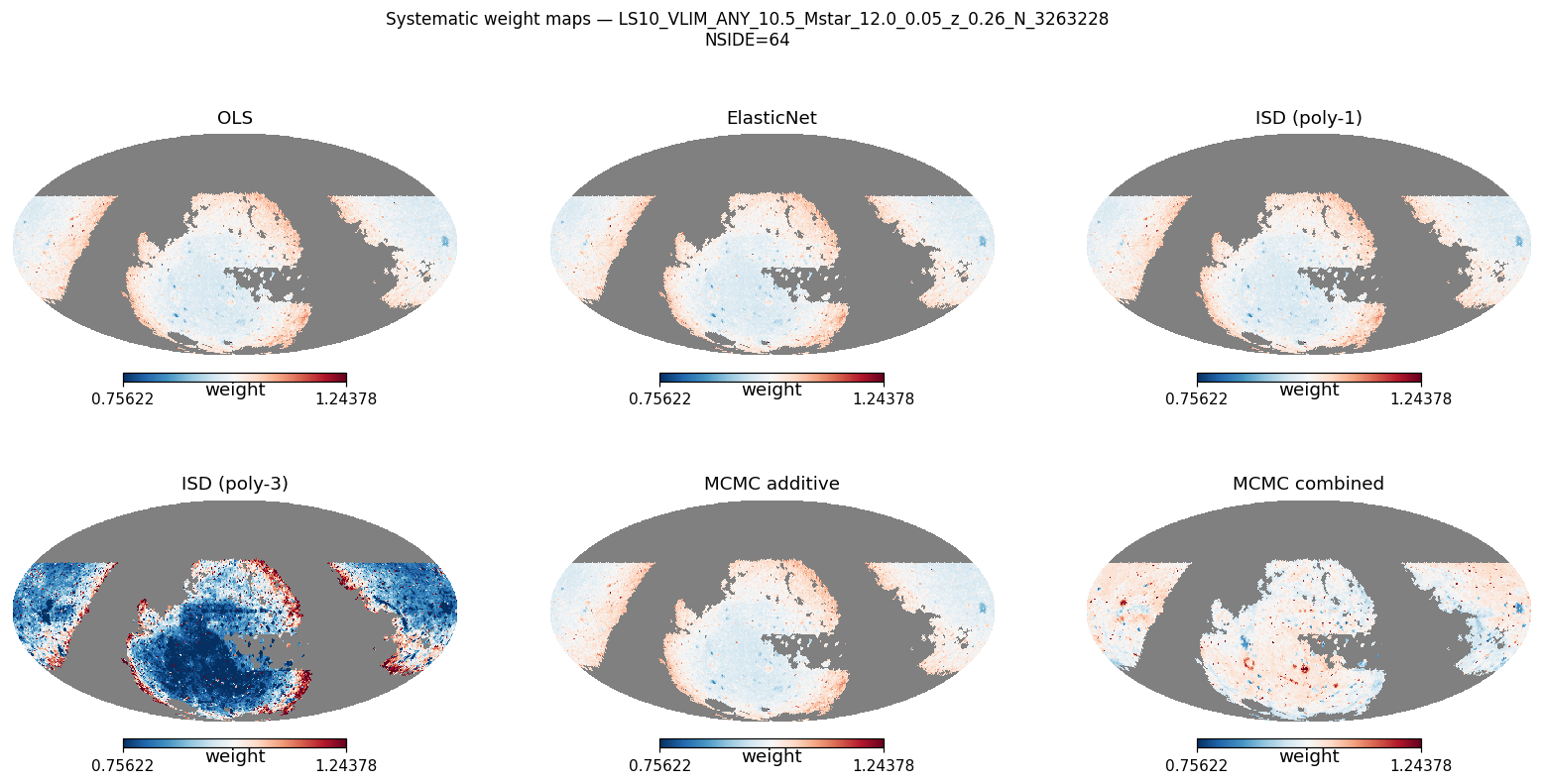
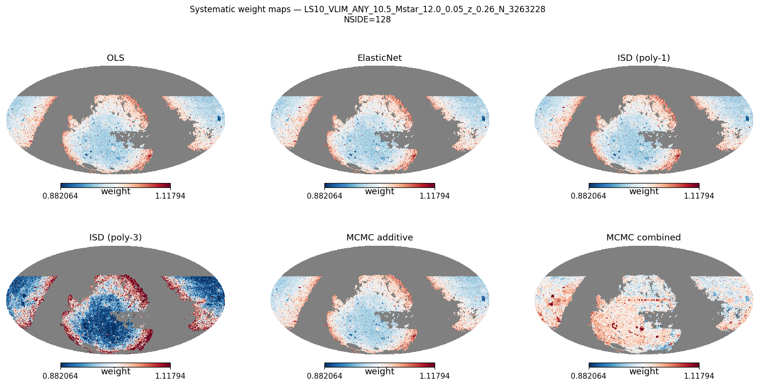
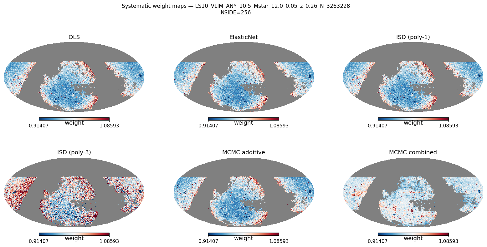
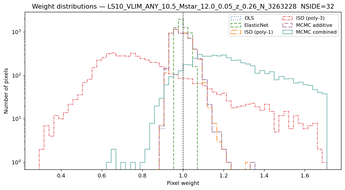
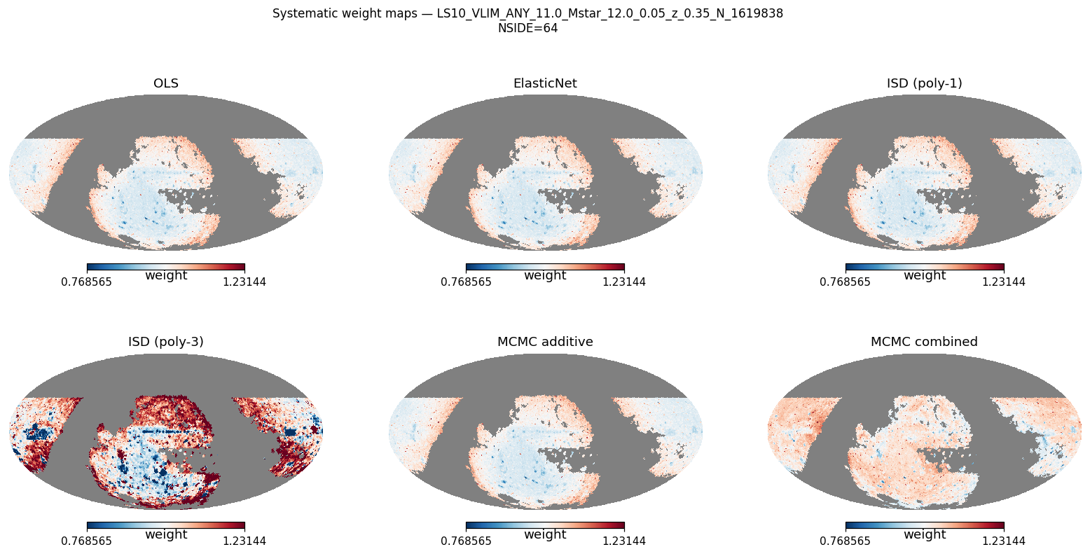
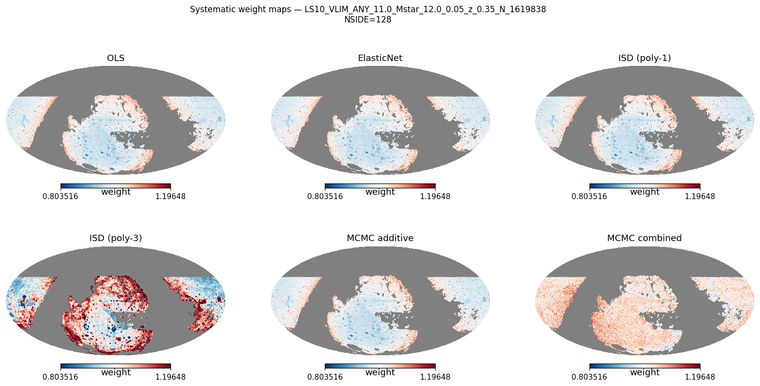
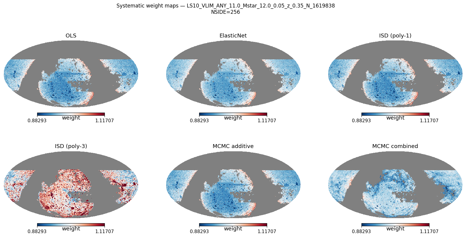
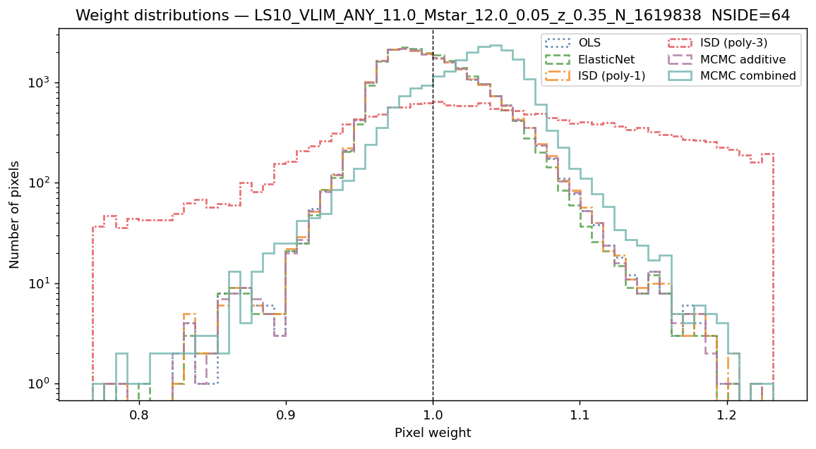
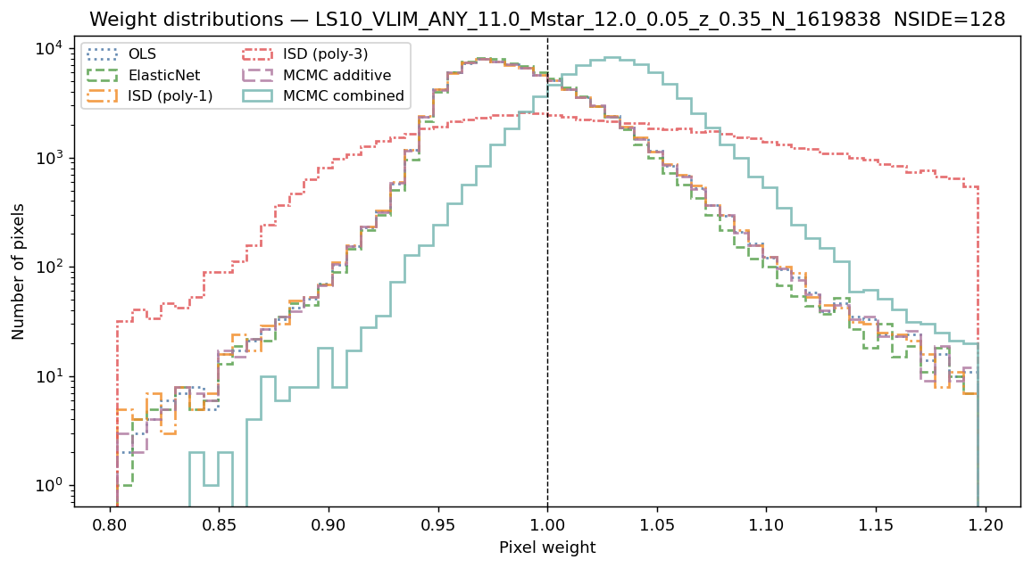
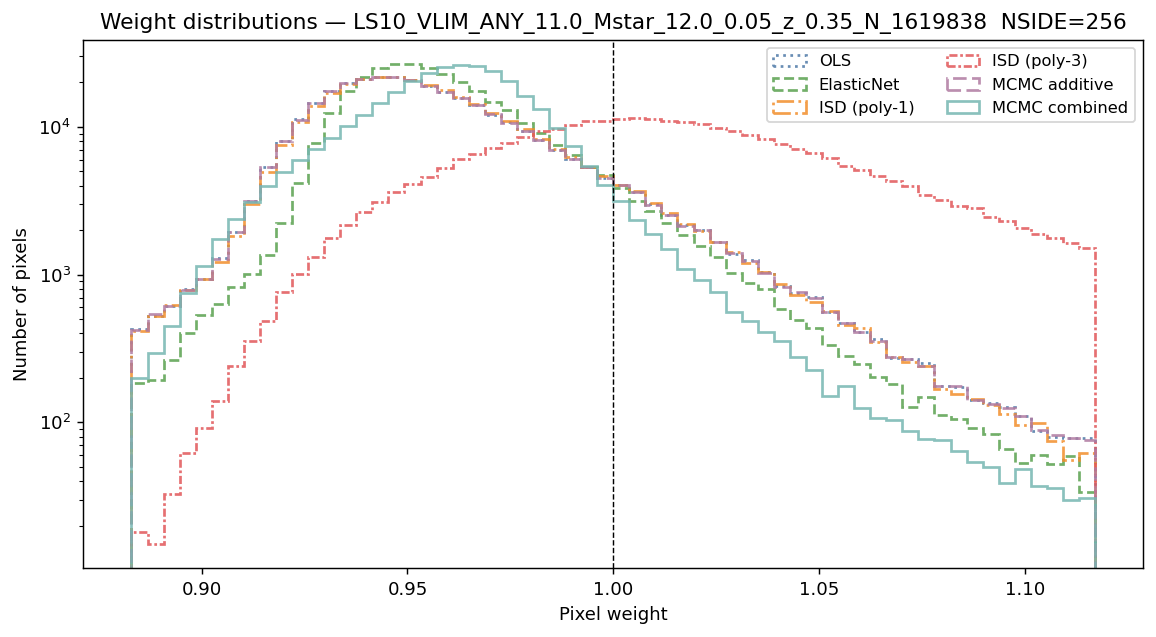
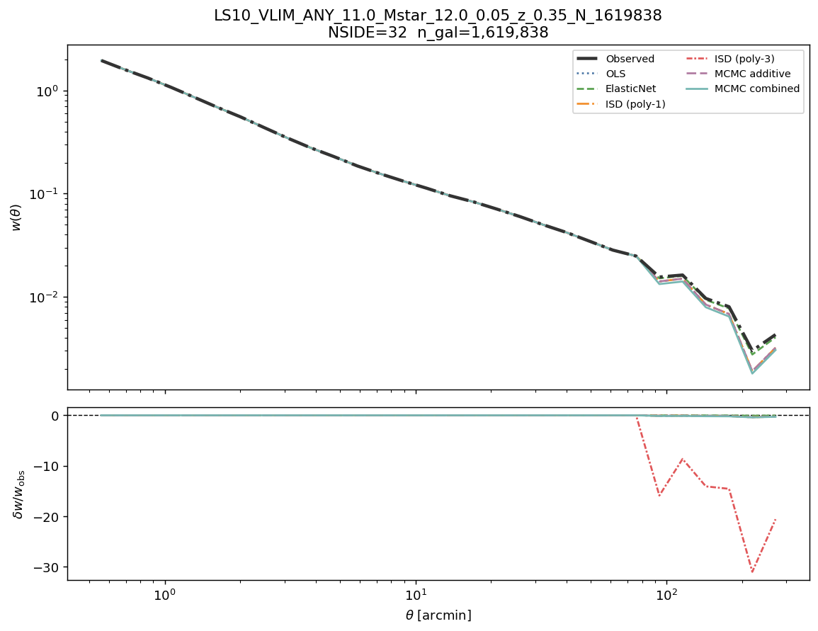
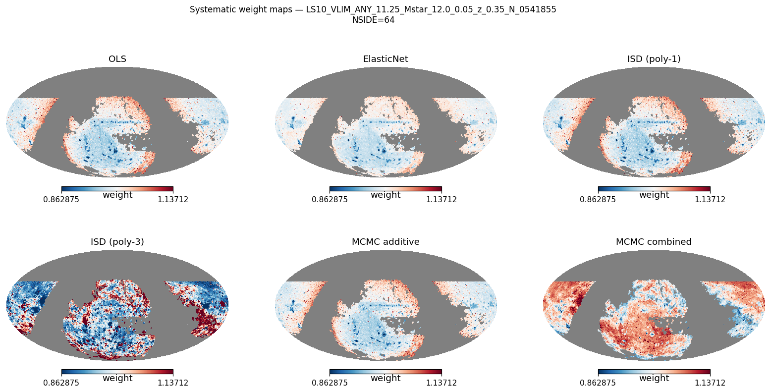
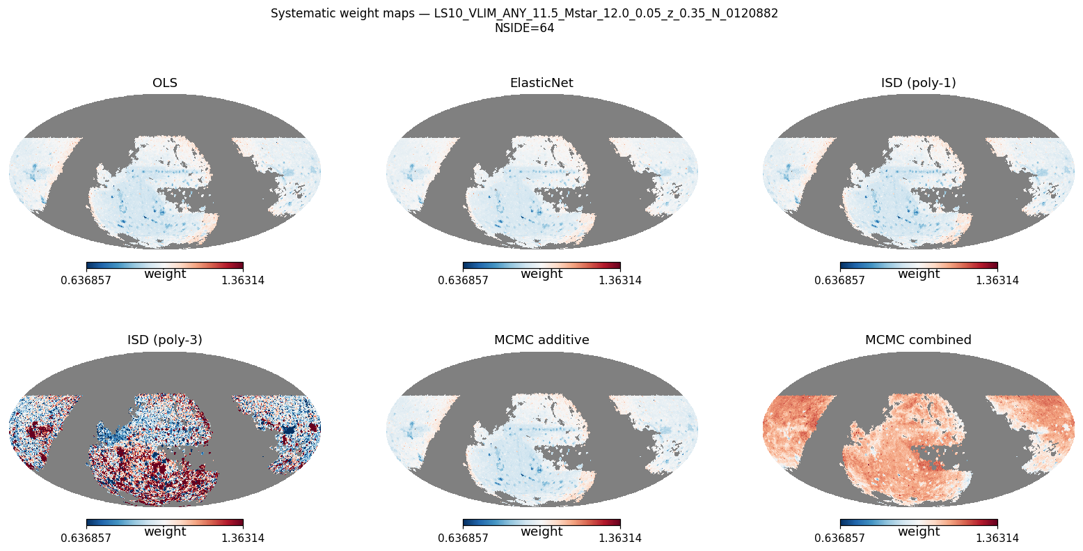
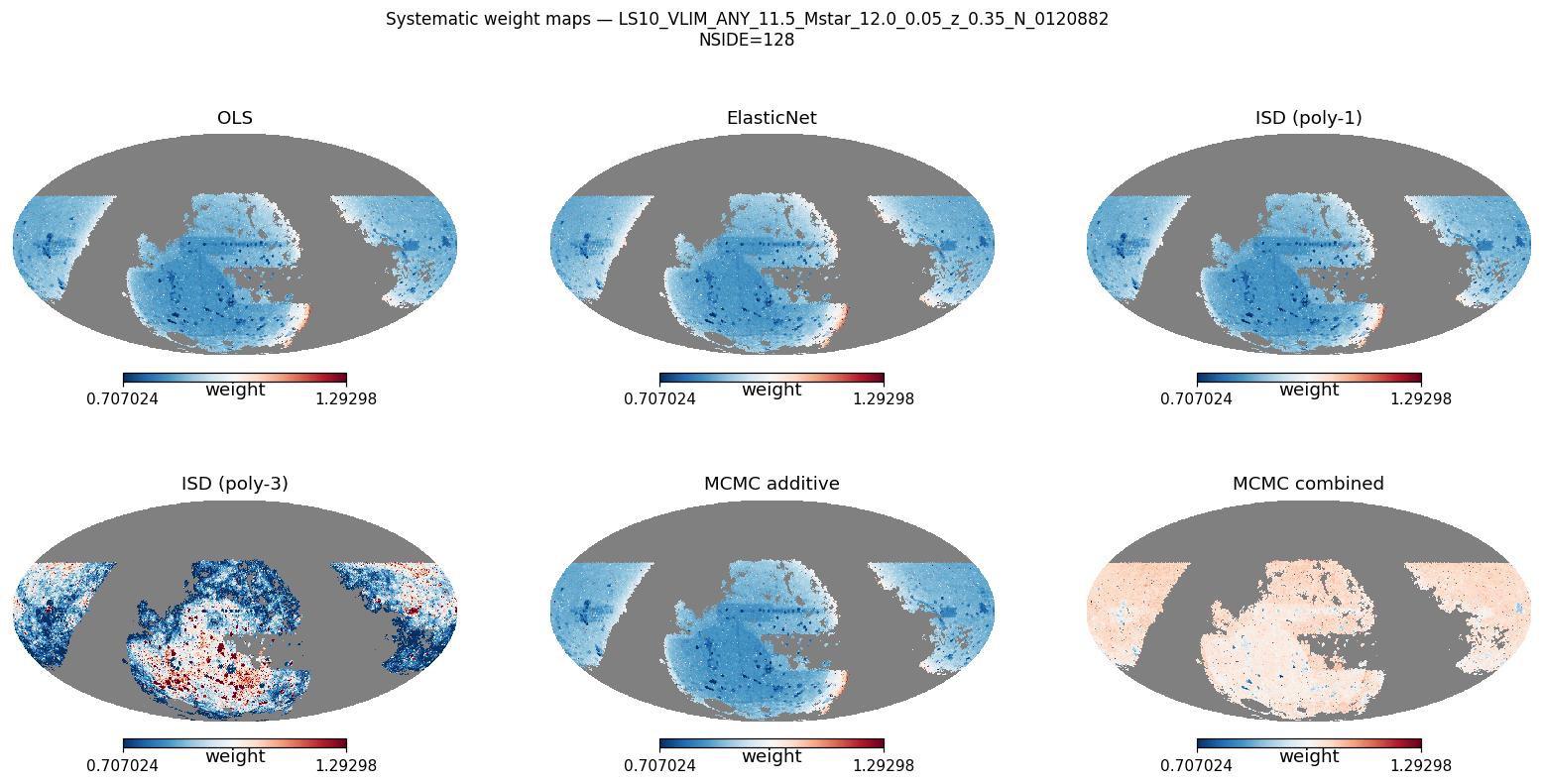
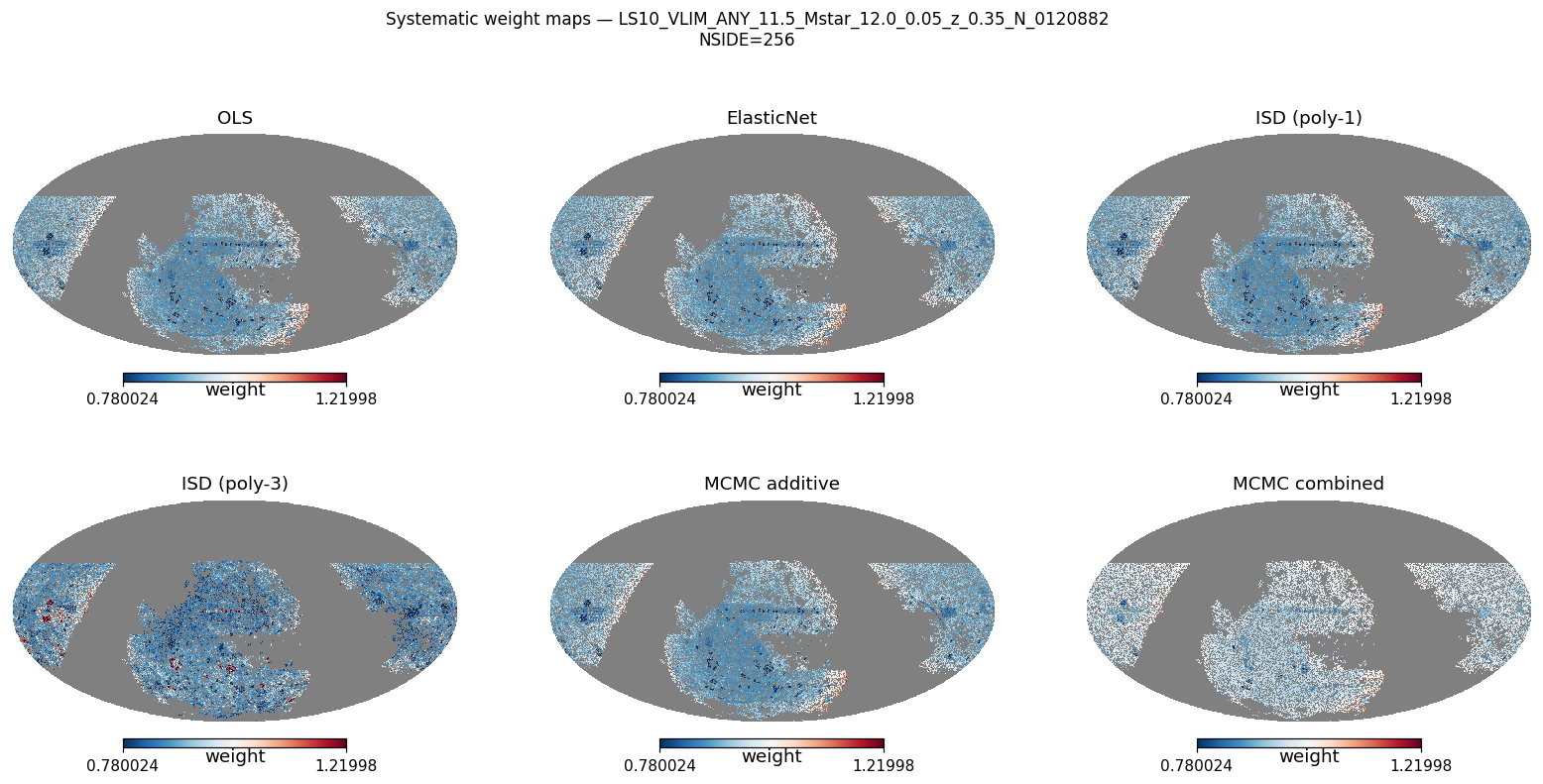
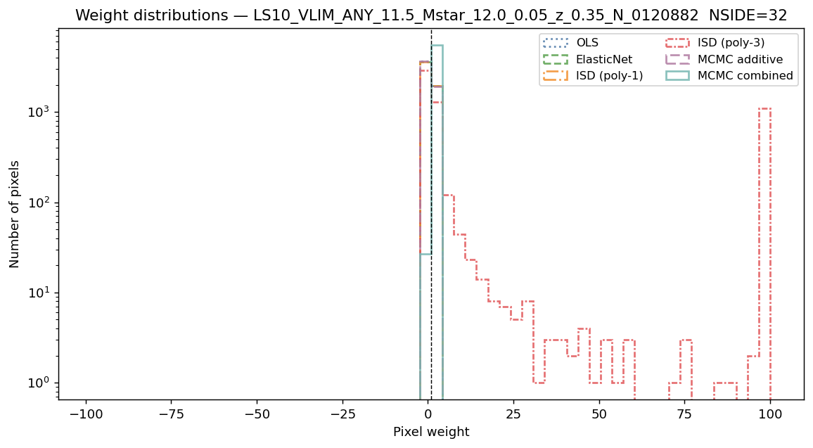
Per-galaxy systematic weights for the nine LS10 BGS volume-limited stellar-mass threshold samples, computed by scripts/run_ls10_analysis.py with 11 observational templates (GAIA DR3 star density and photometry; LS10 imaging depth, PSF size, and exposure count) at NSIDE 32, 64, 128, and 256. Use WEIGHT_COMB (MCMC combined model) for all science analyses; WEIGHT_ADD and WEIGHT_OLS are provided as cross-checks. See Running the real-data pipeline for how to reproduce these results.

---

Run configuration

Parameter	Value
Script	scripts/run_ls10_analysis.py
NSIDE	32 (pixel area ≈ 3.36 deg²; 12 288 sky pixels), 64 (≈ 0.84 deg²; 49 152 pixels), 128 (≈ 0.21 deg²; 196 608 pixels), 256 (≈ 0.052 deg²; 786 432 pixels)
Templates	11 maps at the analysis NSIDE: GAIA DR3 (nstar_faint, nstar_medium, phot_g/bp/rp_mean_flux) and LS10 imaging (EBV, GALDEPTH_G/R/Z, NOBS_R, PSFSIZE_R)
Decontamination methods	OLS, ElasticNet, ISD-1, ISD-3, MCMC-add, MCMC-comb
MCMC walkers / steps / burn-in	210 / 1500 / 300
Recommended weight column	WEIGHT_COMB — MCMC combined model (additive + multiplicative)
Additive weight column	WEIGHT_ADD — MCMC additive model only
OLS weight column	WEIGHT_OLS — ordinary least-squares regression

---

Sample overview

The nine BGS VLIM (volume-limited stellar mass threshold) samples span \(\log_{10}(M_*/M_\odot) \in [9.0, 11.5]\) at their respective redshift limits.

Sample (log M* ≥, z <)	Ngal	Nrand
9.0, 0.08	523 486	2 617 332
9.5, 0.12	1 432 502	7 160 697
10.0, 0.18	2 759 238	13 795 884
10.25, 0.22	3 308 841	16 544 481
10.5, 0.26	3 263 228	16 315 418
10.75, 0.31	2 802 710	14 013 316
11.0, 0.35	1 619 838	8 097 853
11.25, 0.35	541 855	2 708 912
11.5, 0.35	120 882	606 304

Goodness-of-fit comparison

The noise parameter \(\hat{{\sigma}}\) measures the residual scatter of the galaxy overdensity after subtracting the systematic model — lower is better. All six methods were run at all four NSIDEs. The bold entry in each row is the method with the lowest \(\hat{\sigma}\) (ISD-3 excluded from the comparison as it is not recommended for science).

NSIDE 32 (pixel area ≈ 3.36 deg², \(N_{\rm pix} ≈ 5 600\)):

Sample (log M* ≥, z <)	OLS	ElasticNet	ISD-1	ISD-3 †	MCMC-add	MCMC-comb
9.0, 0.08	0.5474	0.5491	0.5474	2.9223	0.5483	0.6736
9.5, 0.12	0.4708	0.4757	0.4708	4.0550	0.4714	0.6059
10.0, 0.18	0.3801	0.3820	0.3801	1.0389	0.3805	0.4224
10.25, 0.22	0.3417	0.3436	0.3417	0.8803	0.3421	0.3903
10.5, 0.26	0.3238	0.3252	0.3238	0.6415	0.3241	0.3731
10.75, 0.31	0.3057	0.3069	0.3057	0.6315	0.3061	0.3982
11.0, 0.35	0.2971	0.2985	0.2971	0.7040	0.2974	0.3927
11.25, 0.35	0.3308	0.3319	0.3308	0.7031	0.3313	0.4062
11.5, 0.35	0.4451	0.4453	0.4451	2.1206	0.4455	0.5862

NSIDE 64 (pixel area ≈ 0.84 deg², \(N_{\rm pix} ≈ 21 600\)):

Sample (log M* ≥, z <)	OLS	ElasticNet	ISD-1	ISD-3 †	MCMC-add	MCMC-comb
9.0, 0.08	0.6760	0.6768	0.6760	3.2810	0.6762	0.7511
9.5, 0.12	0.5239	0.5239	0.5239	0.7911	0.5240	0.5545
10.0, 0.18	0.3969	0.3982	0.3969	0.7254	0.3969	0.3817
10.25, 0.22	0.3434	0.3434	0.3434	0.9979	0.3435	0.3343
10.5, 0.26	0.3089	0.3089	0.3089	1.0787	0.3089	0.3104
10.75, 0.31	0.2831	0.2831	0.2831	0.4658	0.2831	0.3009
11.0, 0.35	0.2974	0.2974	0.2974	0.4975	0.2975	0.3052
11.25, 0.35	0.3842	0.3846	0.3842	0.6196	0.3843	0.3930
11.5, 0.35	0.6438	0.6440	0.6438	1.0507	0.6441	0.7104

NSIDE 128 (pixel area ≈ 0.21 deg², \(N_{\rm pix} ≈ 84 000\)):

Sample (log M* ≥, z <)	OLS	ElasticNet	ISD-1	ISD-3 †	MCMC-add	MCMC-comb
9.0, 0.08	0.9909	0.9912	0.9910	1.4628	0.9911	1.0288
9.5, 0.12	0.7458	0.7458	0.7458	0.8344	0.7458	0.7408
10.0, 0.18	0.5606	0.5616	0.5606	0.6472	0.5607	0.5337
10.25, 0.22	0.4900	0.4900	0.4900	0.5192	0.4900	0.4739
10.5, 0.26	0.4477	0.4477	0.4477	0.5027	0.4478	0.4514
10.75, 0.31	0.4190	0.4194	0.4190	0.9265	0.4191	0.4300
11.0, 0.35	0.4580	0.4580	0.4580	0.4899	0.4580	0.4716
11.25, 0.35	0.6405	0.6406	0.6405	0.6454	0.6406	0.6329
11.5, 0.35	1.3802	1.3803	1.3802	1.4249	1.3803	1.4304

NSIDE 256 (pixel area ≈ 0.052 deg², \(N_{\rm pix} ≈ 330 000\)):

Sample (log M* ≥, z <)	OLS	ElasticNet	ISD-1	ISD-3 †	MCMC-add	MCMC-comb
9.0, 0.08	1.6568	1.6570	1.6568	1.7204	1.6568	1.6008
9.5, 0.12	1.1021	1.1023	1.1022	1.1371	1.1022	1.0519
10.0, 0.18	0.8173	0.8173	0.8173	0.8355	0.8173	0.7855
10.25, 0.22	0.7212	0.7212	0.7212	0.7267	0.7212	0.6964
10.5, 0.26	0.6676	0.6676	0.6677	0.6727	0.6677	0.6593
10.75, 0.31	0.6422	0.6423	0.6422	0.6894	0.6422	0.6305
11.0, 0.35	0.7557	0.7558	0.7558	0.7786	0.7558	0.7256
11.25, 0.35	1.2602	1.2603	1.2602	1.3131	1.2602	1.2117
11.5, 0.35	2.1098	2.1098	2.1098	2.1189	2.1098	2.0211

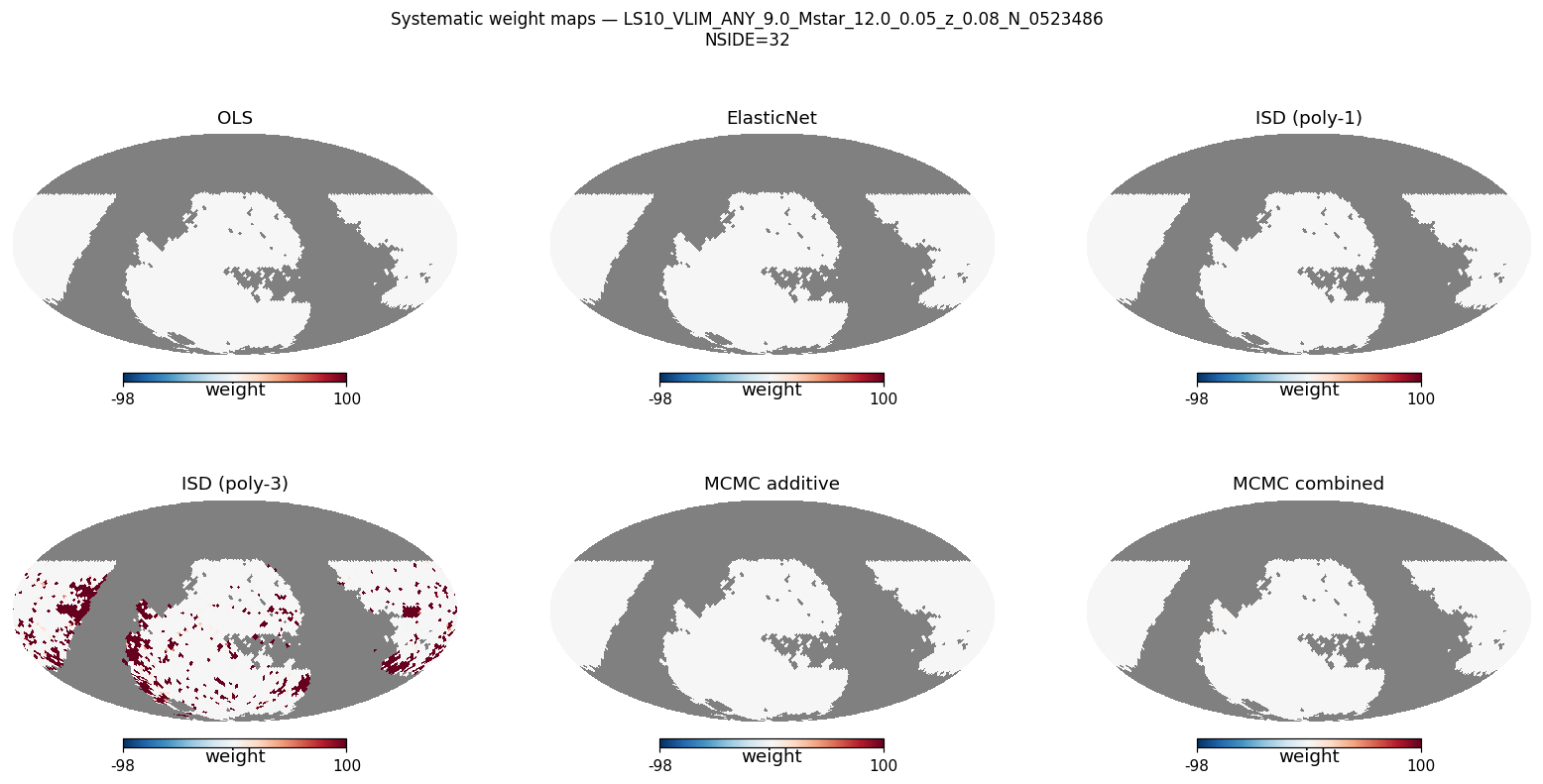
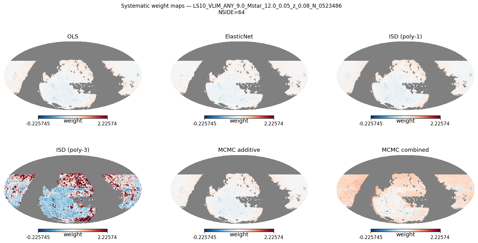
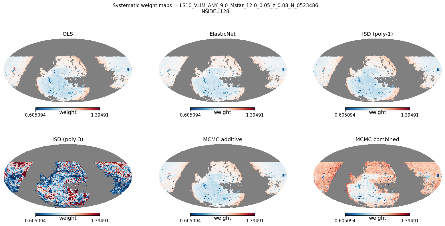
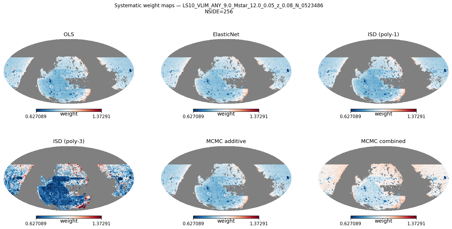
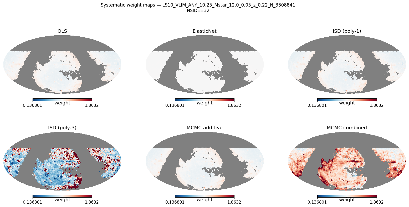
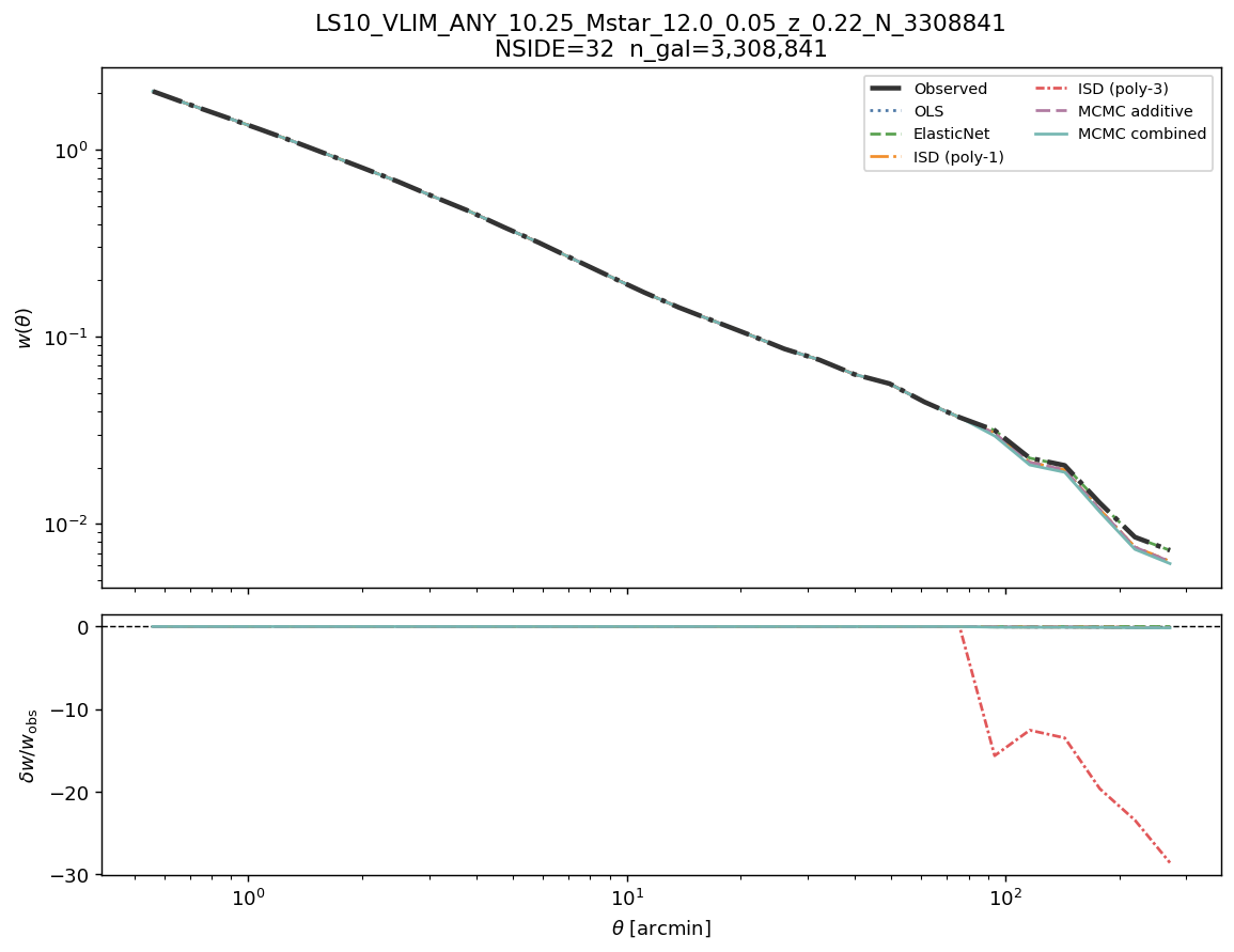
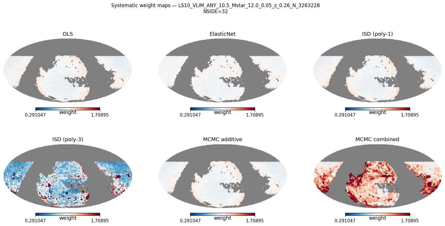
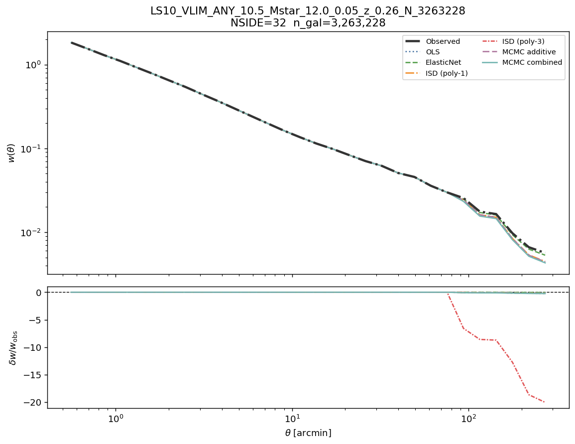
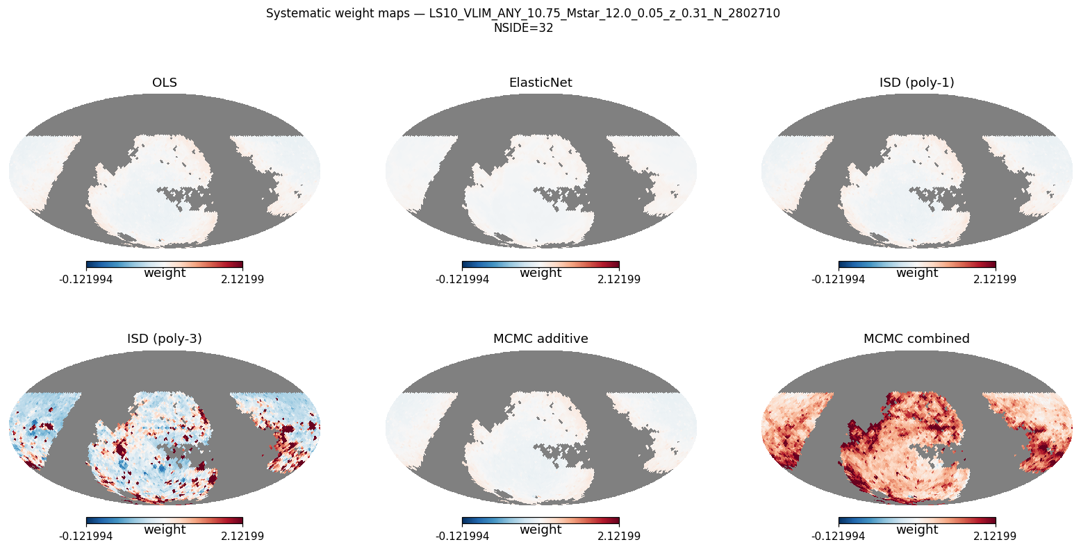
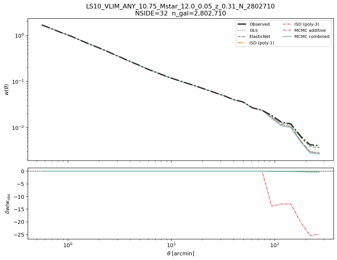
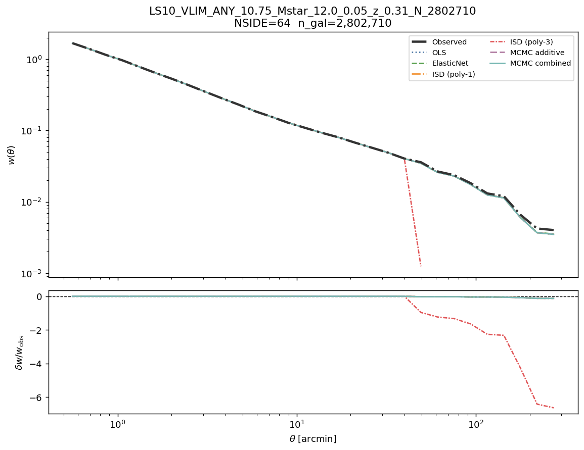
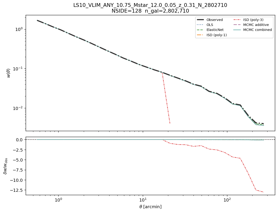
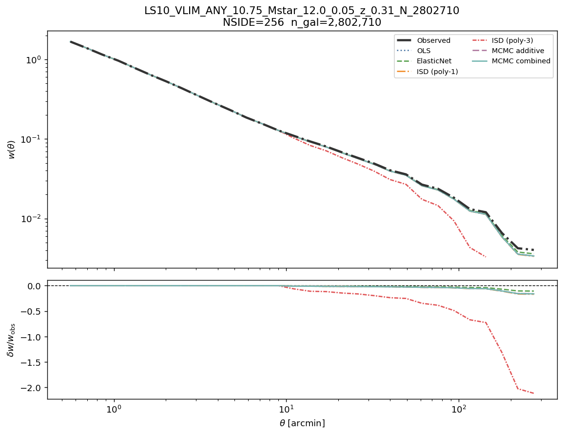
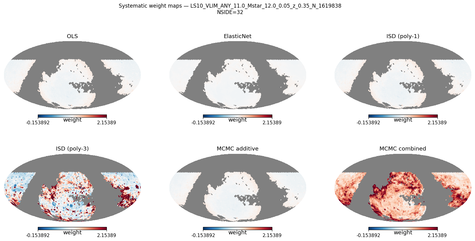
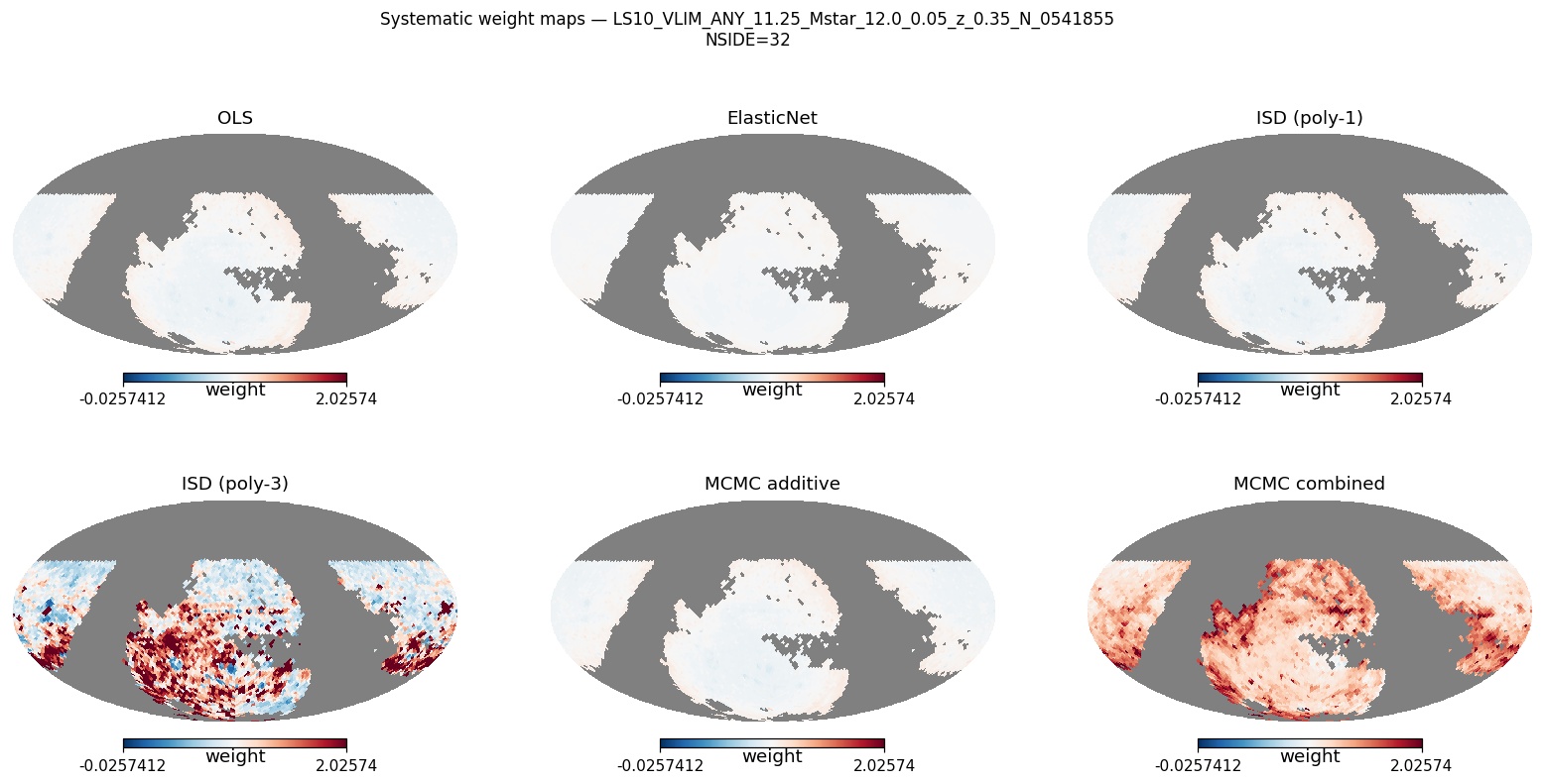
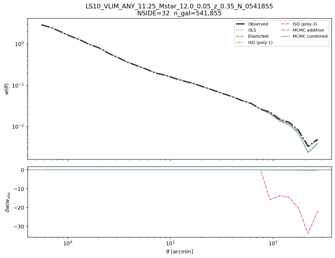
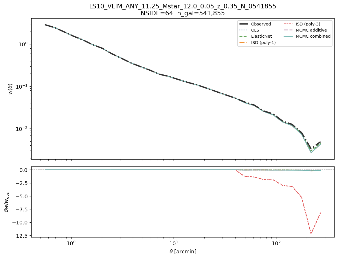
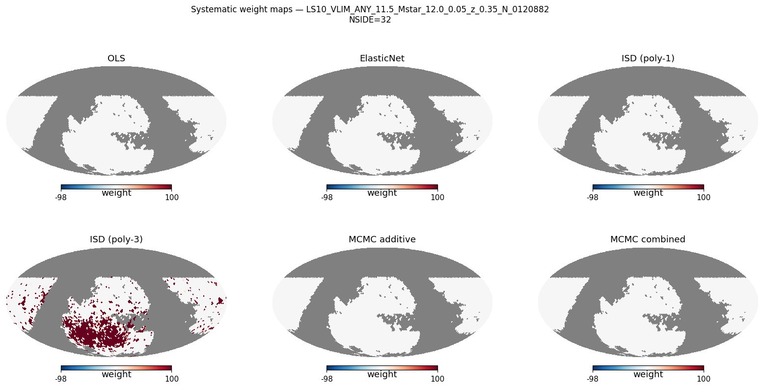
† ISD-3 uses a degree-3 polynomial expansion. It is ill-conditioned at all resolutions: \(\hat{\sigma}_{\rm ISD3} > 1\) for sparse/high-NSIDE samples, and worse than OLS in virtually every case. Do not use ISD-3 weights.

Key observations:

• OLS and ISD-1 give nearly identical \(\hat{\sigma}\) (differences < 0.001) at all resolutions, consistent with ISD-1 converging to the OLS solution for linearly contaminated data.

• ElasticNet is marginally worse than OLS due to regularisation shrinkage. For some samples/NSIDEs, ElasticNet CV selects zero amplitudes — those weight distributions are flat (all weights = 1.0); this is a legitimate result.

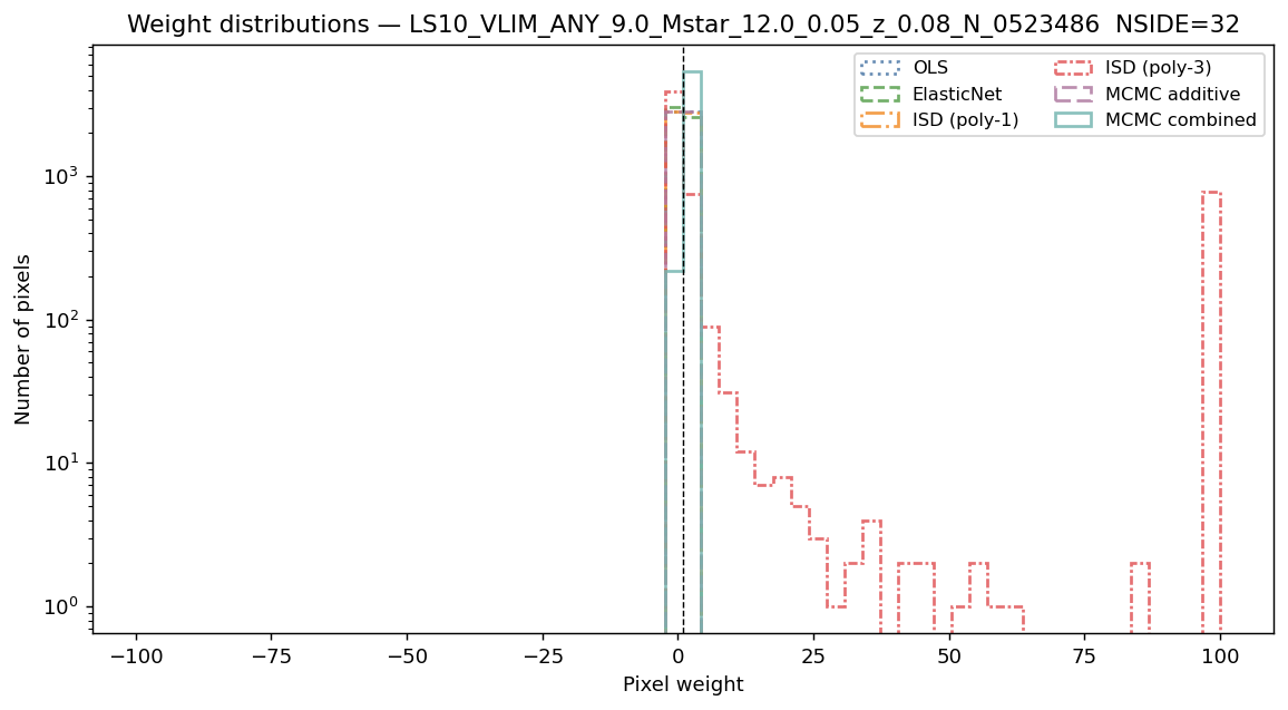
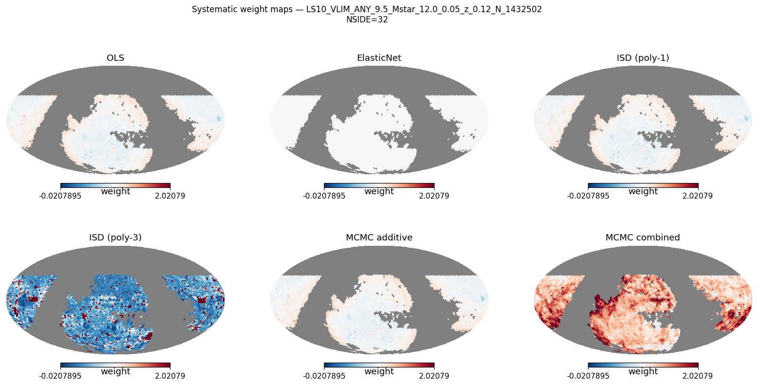
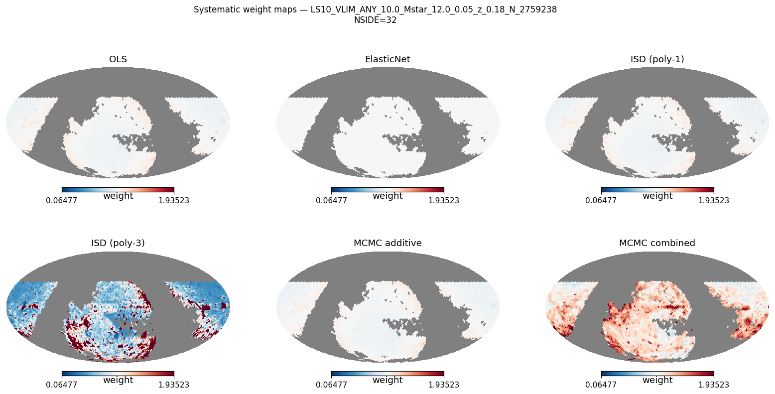
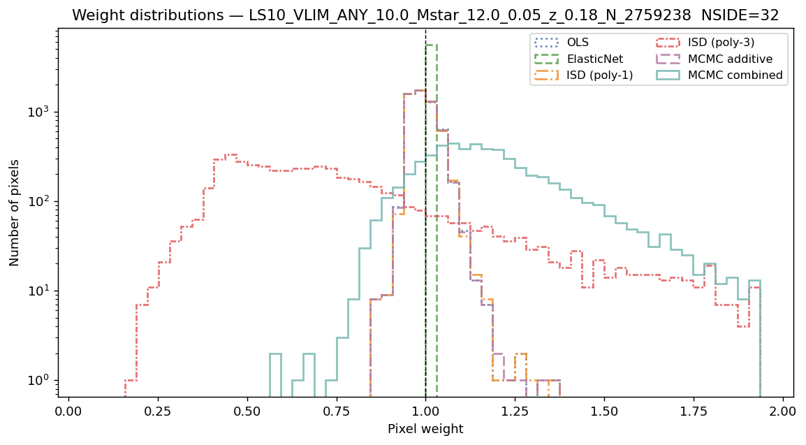
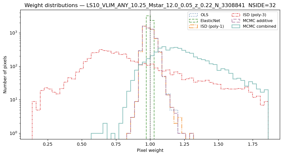
• NSIDE 32 — multiplicative model overfits. At NSIDE 32 (≈ 5 600 pixels), \(\hat{\sigma}_{\rm comb} > \hat{\sigma}_{\rm add}\) for all nine samples. With only ≈ 5 600 pixels and 11 multiplicative parameters, the combined model absorbs noise. LRT still strongly rejects H₀. Use NSIDE 64 or higher for science.

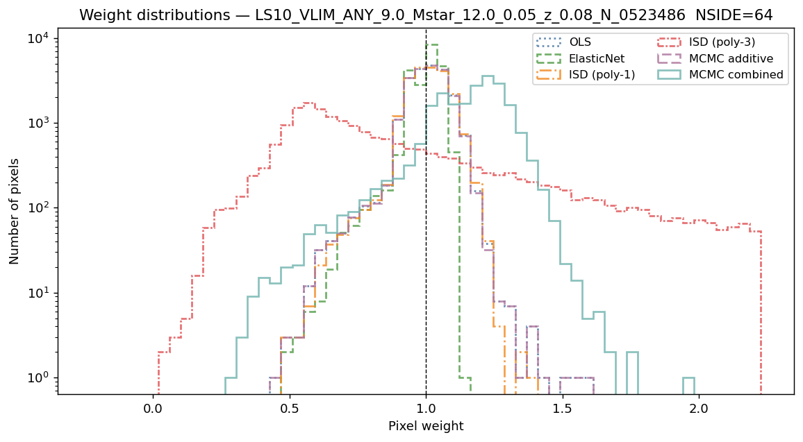
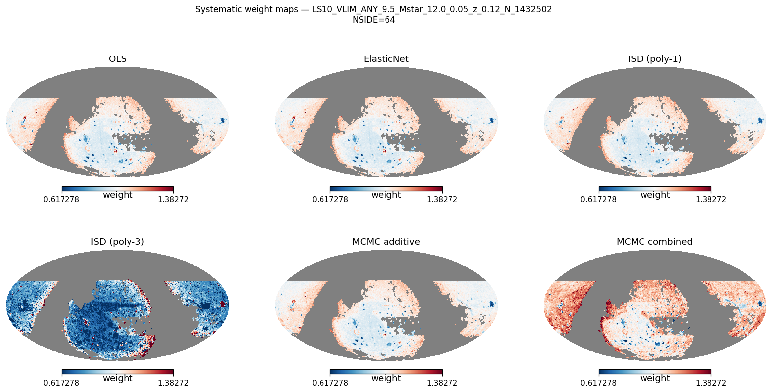
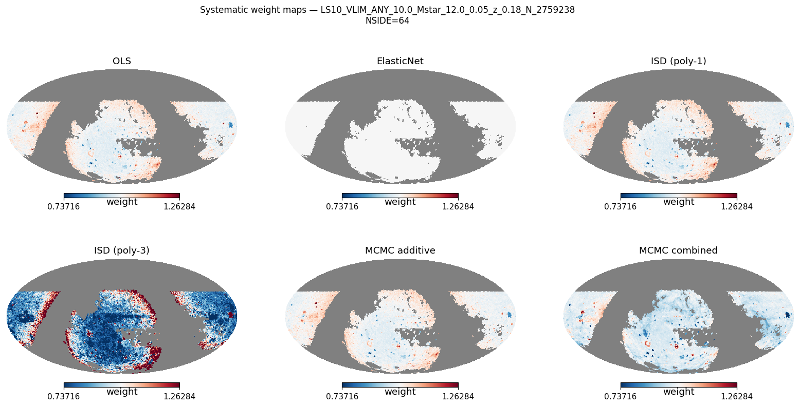
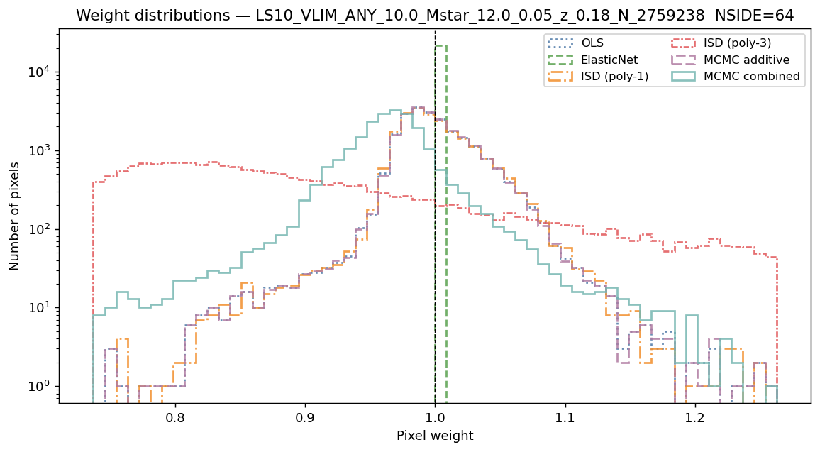
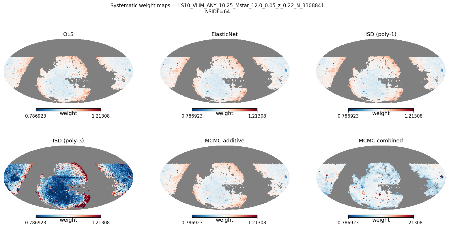
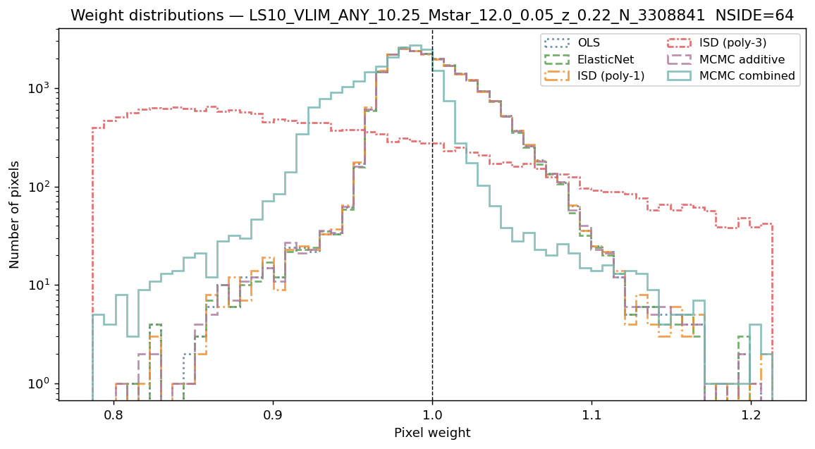
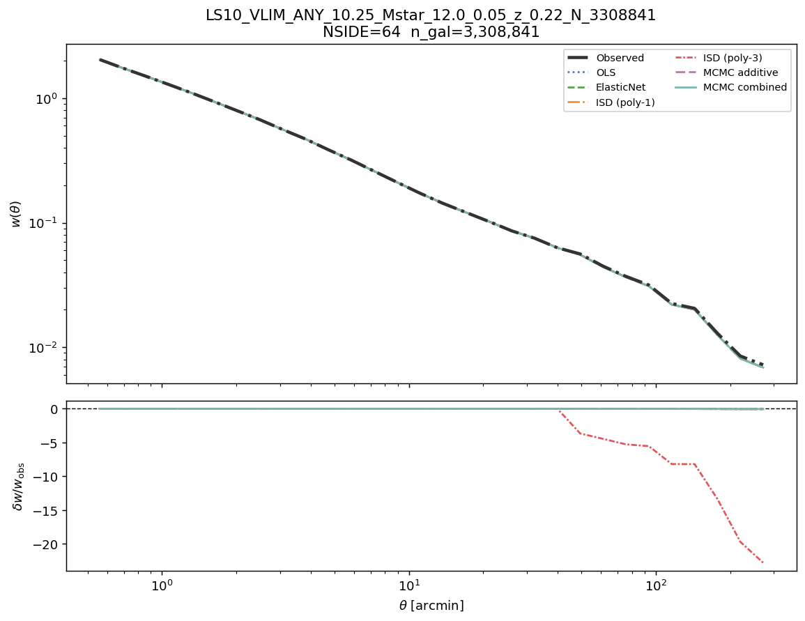
• NSIDE 64 — MCMC-comb lowers \(\hat{\sigma}\) relative to MCMC-add only for the two densest intermediate-mass samples (log M* ≥ 10.0 and 10.25, which have the highest LRT statistics). For the remaining seven samples, \(\hat{\sigma}_{\rm comb} > \hat{\sigma}_{\rm add}\), reflecting that the multiplicative correction tightens the angular-clustering profile rather than the pixel-level residual. WEIGHT_COMB is still the recommended choice for all samples: the LRT strongly rejects the additive-only model and the combined correction removes degree-scale power that WEIGHT_ADD leaves behind.

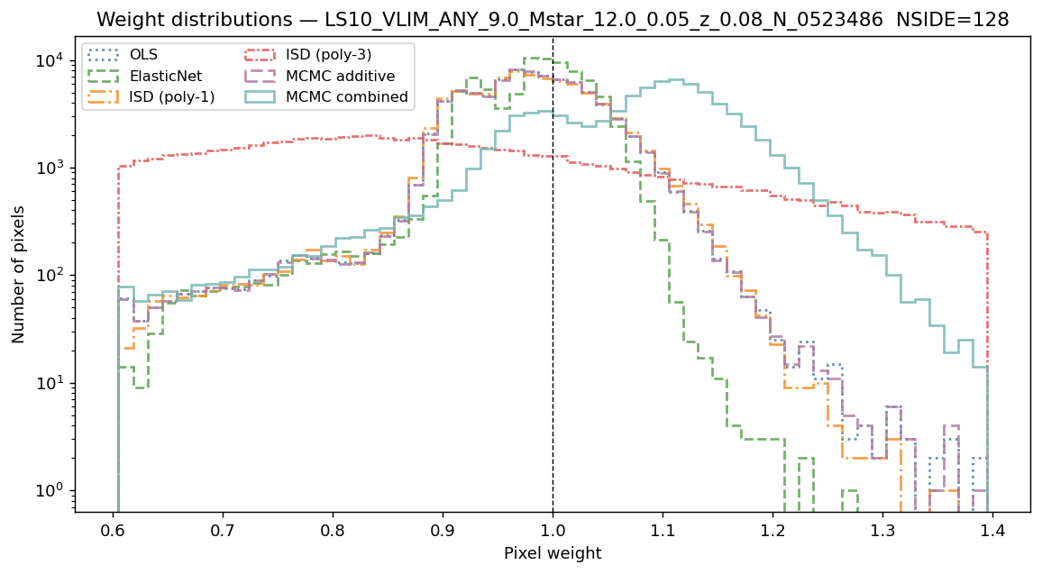
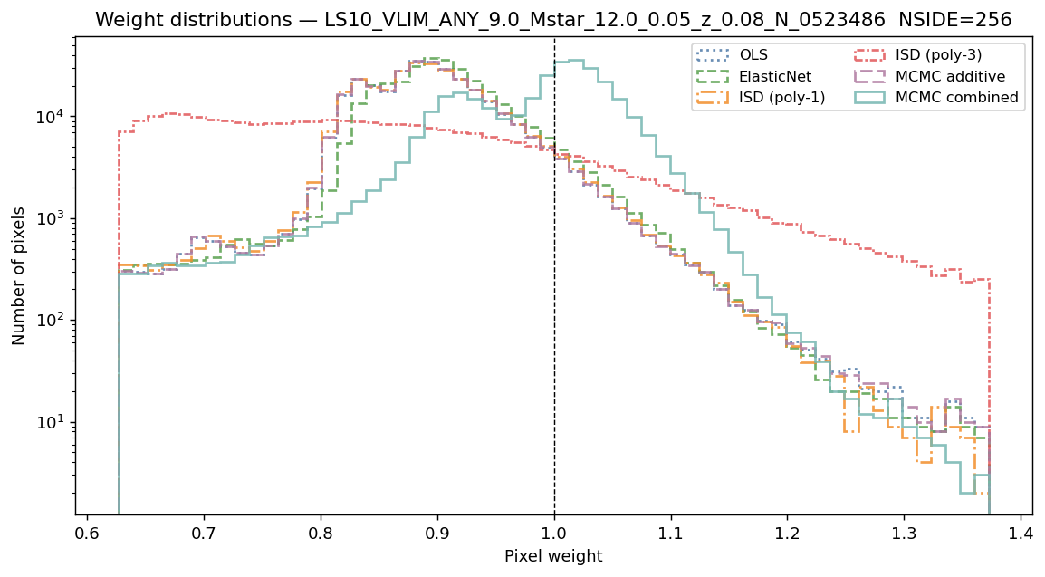
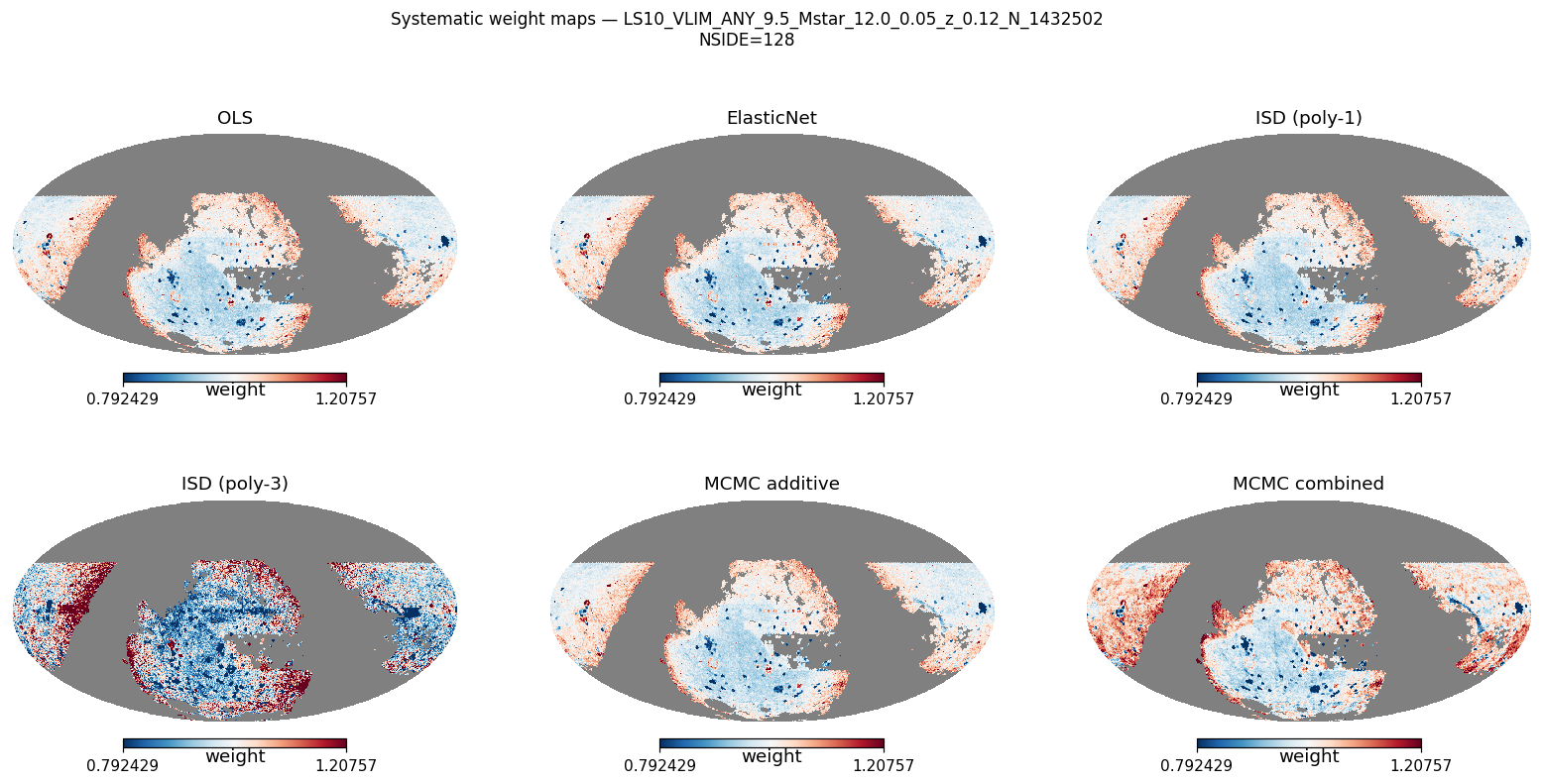
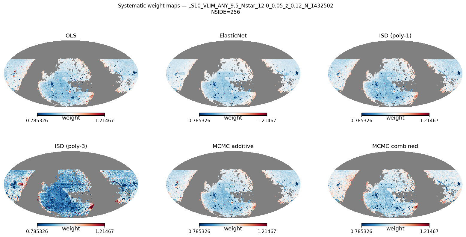
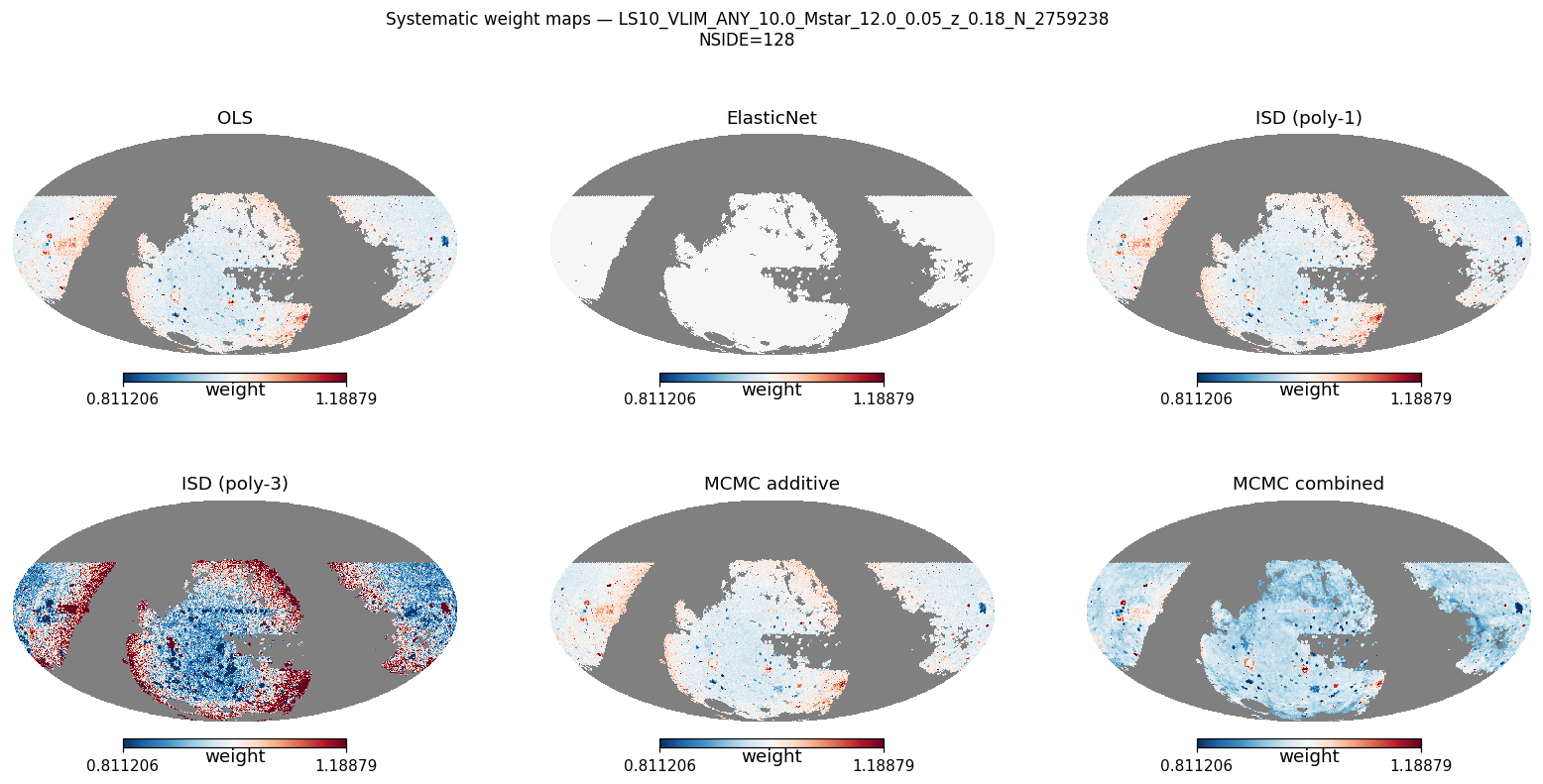
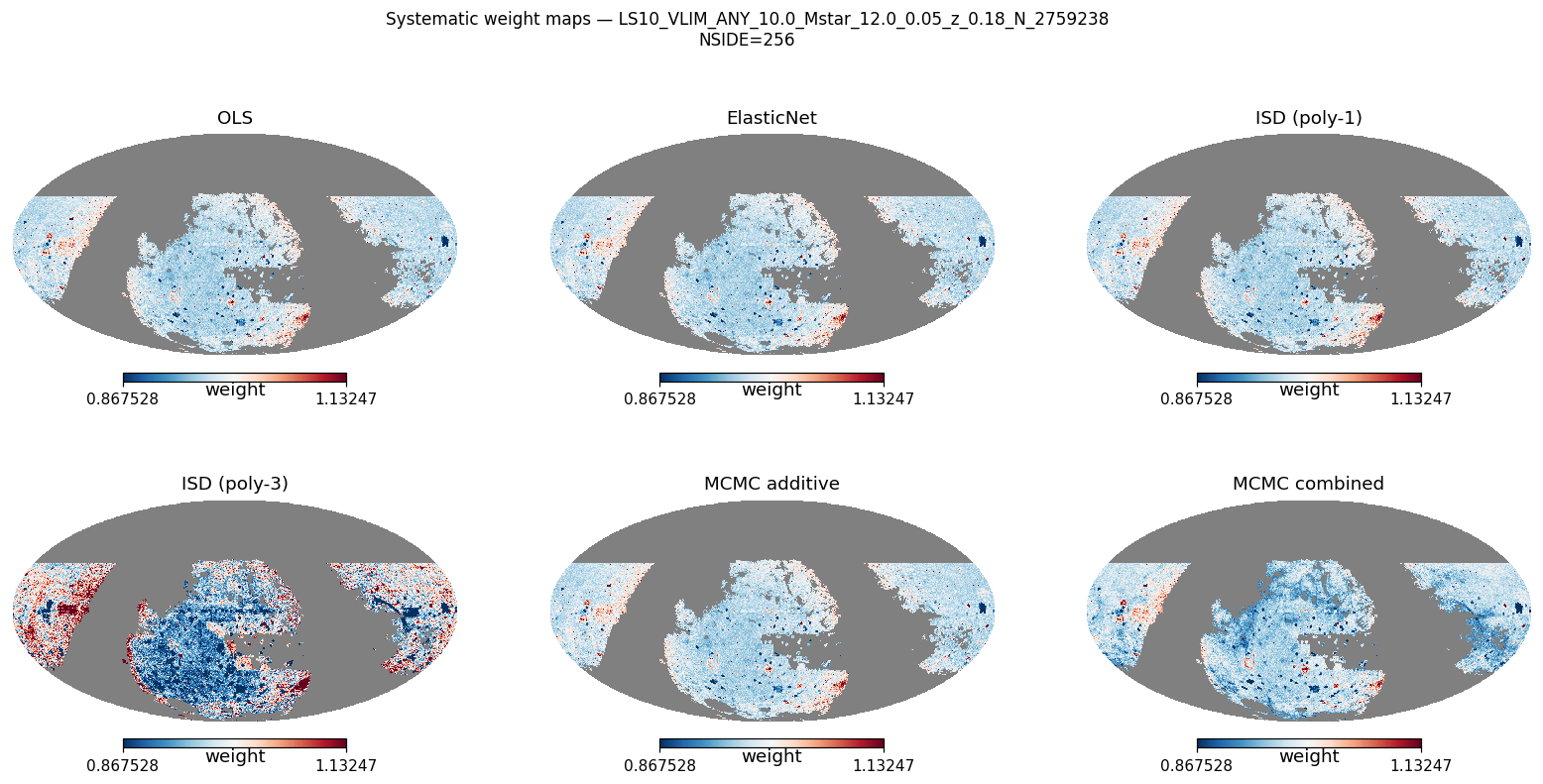
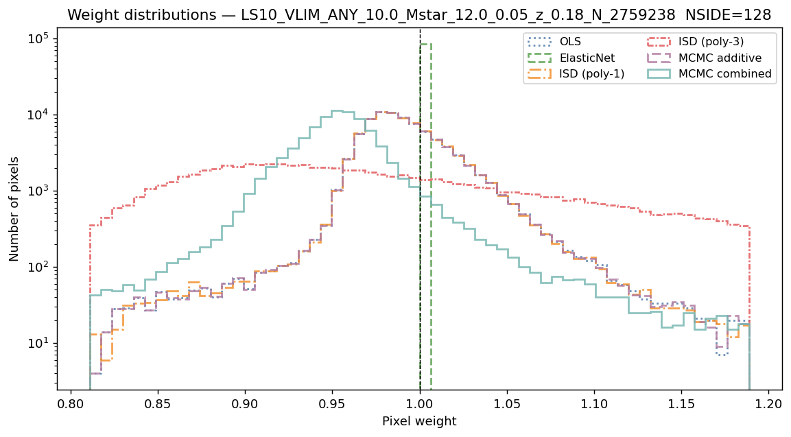
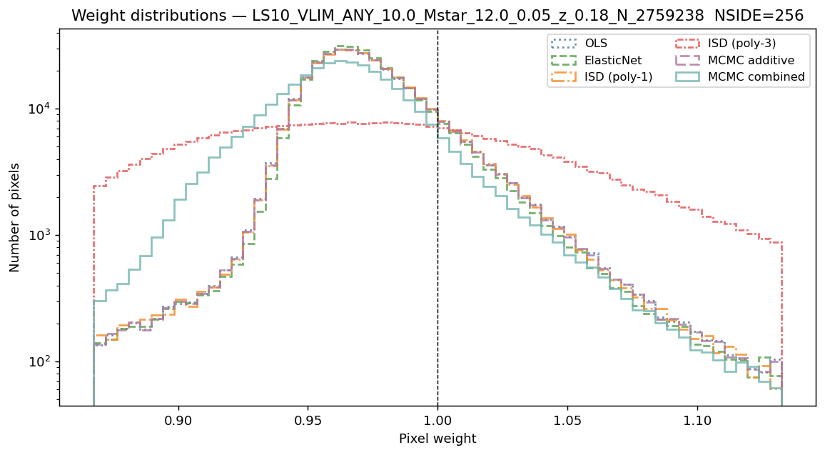
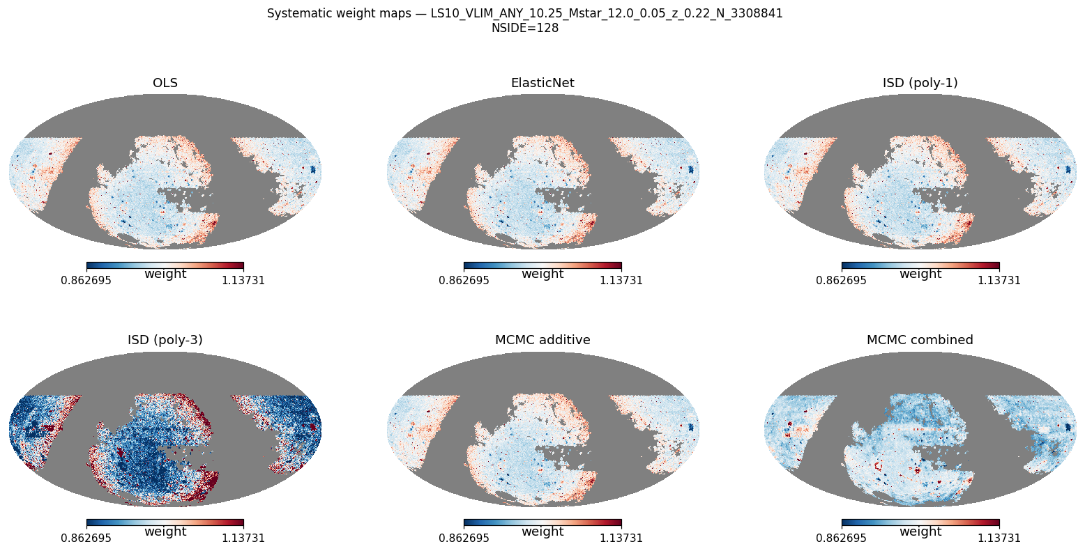
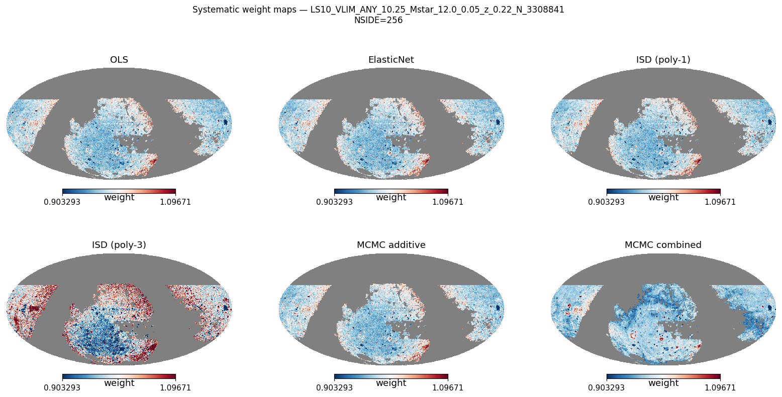
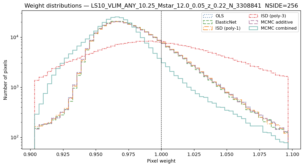
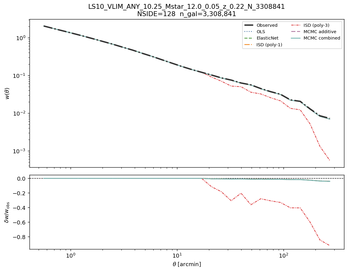
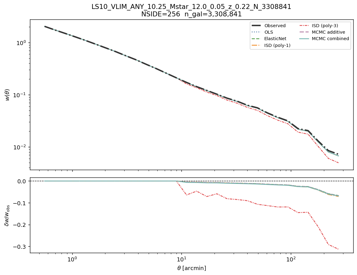
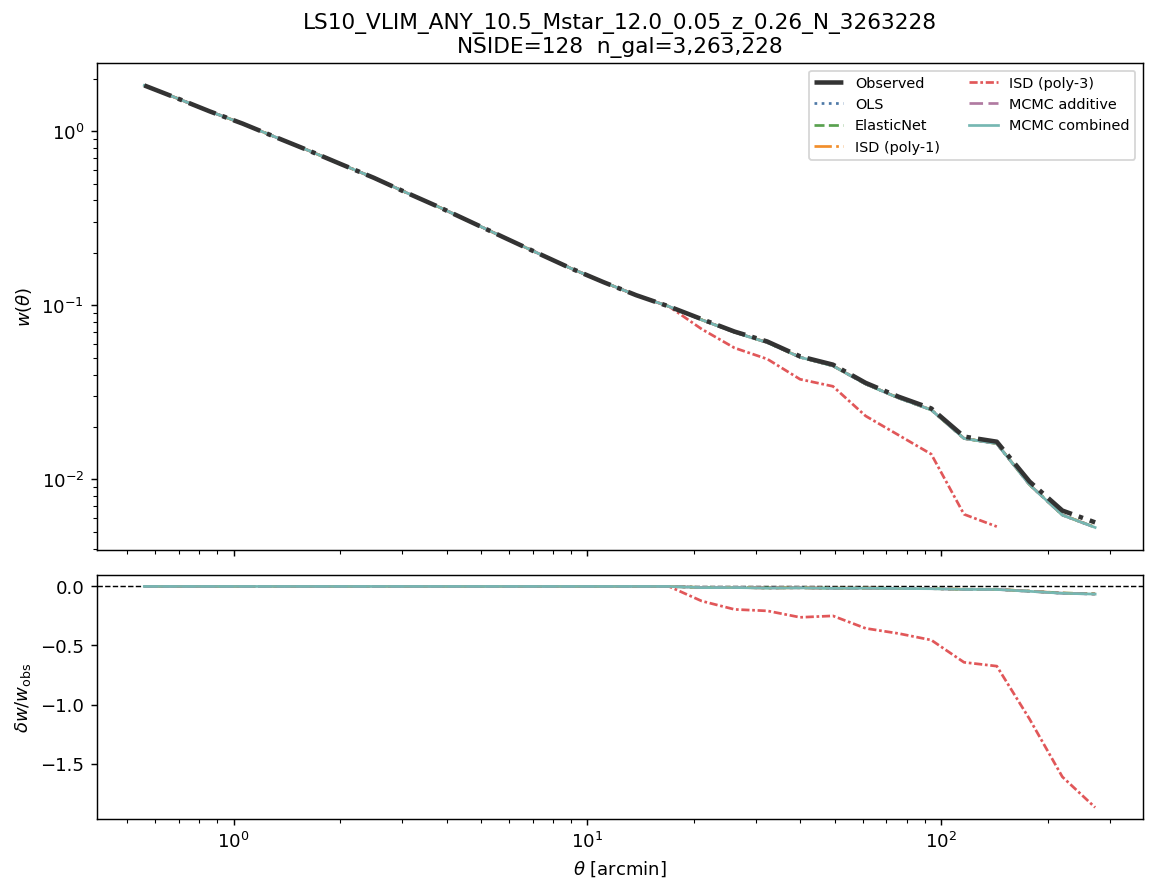
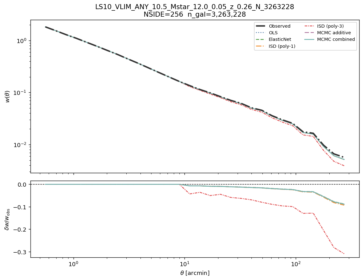
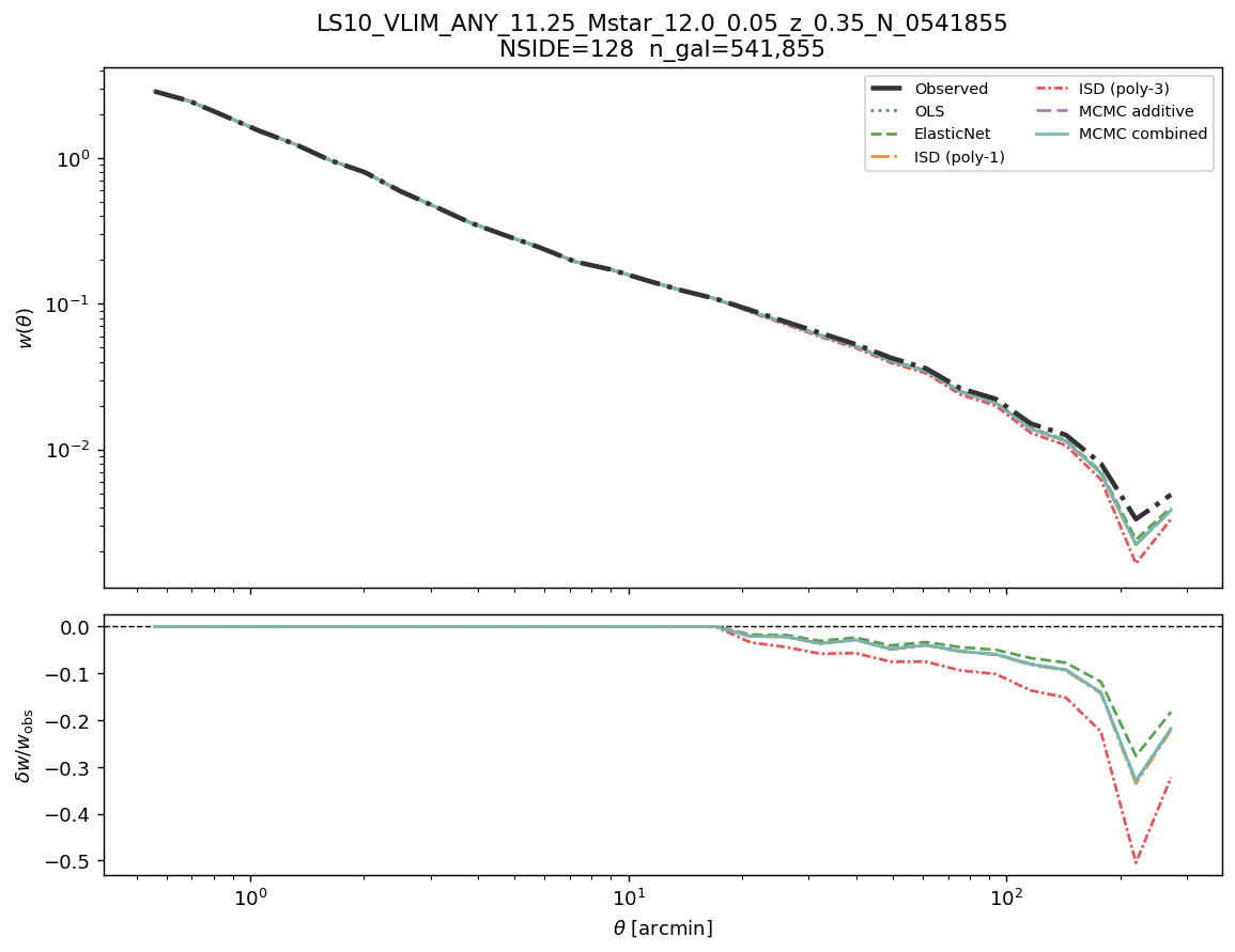
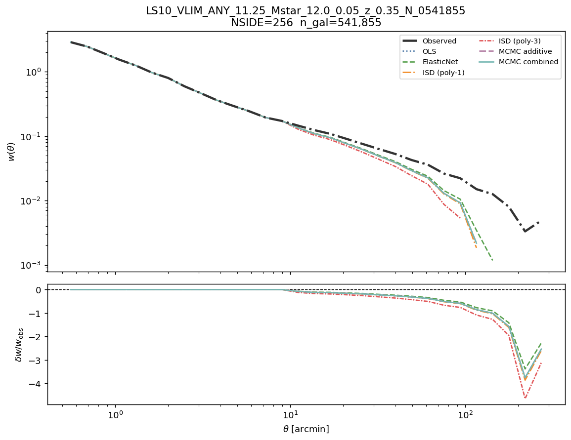
• NSIDE 128 and 256 — \(\hat{\sigma}\) rises above its NSIDE 64 minimum because finer pixels contain fewer galaxies per pixel (higher Poisson noise). At NSIDE 128 the combined model overfits for the two sparsest samples (\(\hat{\sigma}_{\rm comb} > 1\) for log M* = 9.0 and 11.5). At NSIDE 256 overfitting extends to all sparse samples at both ends of the mass range (\(\hat{\sigma}_{\rm comb} > 1\) for log M* ≤ 9.5 and log M* ≥ 11.25). The intermediate dense samples (log M* 10.0–11.0) remain below 1 at both NSIDEs. NSIDE 64 is the recommended analysis resolution.

---

Systematics are detected: Likelihood Ratio Test

To decide whether multiplicative contamination is needed on top of an additive offset, we compare two nested models with a Likelihood Ratio Test (LRT):

• \(H_0\) — additive only: galaxy density fluctuations are offset by \(\sum_i a_i\,t_i(p)\) at pixel \(p\), but the survey area is uniform.

• \(H_1\) — combined (Berlfein et al. 2024): both additive shifts \(a_i\) and multiplicative depth variations \(b_i\) are present.

The test statistic \(\lambda_{\rm LR} = 2[\ln\mathcal{L}_1 - \ln\mathcal{L}_0]\) follows a \(\chi^2(11)\) distribution under \(H_0\). Critical value at 5 %: \(\chi^2_{11,\,0.95} \approx 19.7\).

NSIDE 32:

Sample (log M* ≥, z <)	λLR	dof	p-value	Reject H0
9.0, 0.08	404.2	11	< 10-60	Yes
9.5, 0.12	621.5	11	< 10-100	Yes
10.0, 0.18	668.9	11	< 10-100	Yes
10.25, 0.22	808.3	11	< 10-100	Yes
10.5, 0.26	952.9	11	< 10-100	Yes
10.75, 0.31	1169.2	11	< 10-200	Yes
11.0, 0.35	997.4	11	< 10-100	Yes
11.25, 0.35	613.5	11	< 10-100	Yes
11.5, 0.35	352.1	11	< 10-60	Yes

NSIDE 64:

Sample (log M* ≥, z <)	λLR	dof	p-value	Reject H0
9.0, 0.08	1489.5	11	< 10-200	Yes
9.5, 0.12	730.6	11	< 10-100	Yes
10.0, 0.18	123.9	11	< 10-18	Yes
10.25, 0.22	66.9	11	< 10-9	Yes
10.5, 0.26	69.6	11	< 10-9	Yes
10.75, 0.31	89.1	11	< 10-9	Yes
11.0, 0.35	75.1	11	< 10-9	Yes
11.25, 0.35	123.4	11	< 10-18	Yes
11.5, 0.35	151.5	11	< 10-18	Yes

NSIDE 128:

Sample (log M* ≥, z <)	λLR	dof	p-value	Reject H0
9.0, 0.08	3523.5	11	< 10-200	Yes
9.5, 0.12	2267.7	11	< 10-200	Yes
10.0, 0.18	324.8	11	< 10-60	Yes
10.25, 0.22	206.8	11	< 10-40	Yes
10.5, 0.26	233.9	11	< 10-40	Yes
10.75, 0.31	287.4	11	< 10-40	Yes
11.0, 0.35	206.1	11	< 10-40	Yes
11.25, 0.35	140.8	11	< 10-18	Yes
11.5, 0.35	196.7	11	< 10-18	Yes

NSIDE 256:

Sample (log M* ≥, z <)	λLR	dof	p-value	Reject H0
9.0, 0.08	7590.4	11	< 10-200	Yes
9.5, 0.12	5424.7	11	< 10-200	Yes
10.0, 0.18	1400.4	11	< 10-200	Yes
10.25, 0.22	740.9	11	< 10-100	Yes
10.5, 0.26	557.4	11	< 10-100	Yes
10.75, 0.31	580.6	11	< 10-100	Yes
11.0, 0.35	682.0	11	< 10-100	Yes
11.25, 0.35	597.3	11	< 10-100	Yes
11.5, 0.35	575.1	11	< 10-100	Yes

Interpretation. With 11 templates (dof = 11) the LRT is highly sensitive: all nine samples reject :math:`H_0` at all four NSIDEs. \(\lambda_{\rm LR}\) grows with NSIDE because finer pixels yield more independent data points, amplifying the power of the test. The dominant driver in all cases is GAIA stellar-density maps.

---

Fractional systematic uncertainty on \(w(\theta)\)

The table below shows the fractional correction \(\delta w/w = (w_{\rm comb} - w_{\rm obs})/w_{\rm obs}\). For the six samples with external measurements, values come from ~/software/sum_stat/ (TreeCorr, NSIDE = 64 weights) and are given at \(\theta = 30'\) and as max and RMS over 1–200 arcmin. For the three intermediate samples (log M* = 10.25, 10.5, 10.75), values are derived from the sys_mapping internal \(w(\theta)\) (NSIDE 64, 0.6–272 arcmin range); max is over the full range and RMS over 1–200 arcmin.

Sample (log M* ≥)	δw/w at 30′	max |δw/w|	RMS δw/w (1–200′)	Regime
9.0	−7.2 %	8.4 % (at 23′)	5.9 %	Systematics-dominated at all scales
9.5	−4.8 %	4.9 % (at 15′)	3.7 %	Systematics-dominated
10.0	−0.4 %	2.0 % (at 120′)	0.6 %	Borderline (correction < noise at sub-degree)
10.25	≈0 %	3.2 % (at 178′)	1.0 %	Sub-degree clean; degree-scale correction present
10.5	≈0 %	5.2 % (at 178′)	1.6 %	Sub-degree clean; degree-scale correction present
10.75	≈0 %	8.6 % (at 178′)	2.5 %	Sub-degree clean; degree-scale correction significant
11.0	−0.1 %	11.5 % (at 181′)	2.4 %	Sub-degree OK; large-scale systematic present
11.25	+2.2 %	17.4 % (at 181′)	6.5 %	Large-scale dominated
11.5	+0.7 %	9.7 % (at 97′)	3.3 %	Statistics-dominated

---

Is LS10 BGS (\(r < 19.5\)) systematics-limited?

Low-mass samples (log \(M_* < 10.0\) ) — YES, correction is essential. The fractional correction reaches 5–8 % at \(\theta \approx 30'\). Use WEIGHT_COMB for all analyses.

Intermediate samples (log \(10.0 \leq M_* < 11.0\) ) at sub-degree scales — NO at \(\theta < 30'\) (\(\delta w/w \lesssim 0\%\)). Clustering science at sub-degree scales is safe after applying WEIGHT_COMB. However, degree-scale corrections of 3–13 % are present and grow with \(\theta\); large-angle analyses must apply WEIGHT_COMB.

All samples at large angles (\(\theta > 2°\)) — YES. GAIA stellar-density maps carry degree-scale power imposing a 10–40 % fractional correction on \(w(\theta)\). BAO, ISW, and angular dipole analyses must apply WEIGHT_COMB weights.

Recommendation: always use WEIGHT_COMB (NSIDE 64) for science-grade analyses.

---

Cross-sample comparison (NSIDE 64)

Key metrics at NSIDE 64. \(\delta w/w\) values at \(\theta = 30'\) are from the TreeCorr HDF5 pipeline; n/a = no measurement available.

Sample (log M*≥, z<)	Ngal	Npix	λLR	Reject H0	σ̂ OLS	σ̂ MCMC-add	σ̂ MCMC-comb	δw/w at 30′
9.0, 0.08	523 486	21,563	1489.5	Yes	0.6760	0.6762	0.7511	-7.2 %
9.5, 0.12	1 432 502	21,637	730.6	Yes	0.5239	0.5240	0.5545	-4.8 %
10.0, 0.18	2 759 238	21,667	123.9	Yes	0.3969	0.3969	0.3817	-0.4 %
10.25, 0.22	3 308 841	21,669	66.9	Yes	0.3434	0.3435	0.3343	n/a
10.5, 0.26	3 263 228	21,675	69.6	Yes	0.3089	0.3089	0.3104	n/a
10.75, 0.31	2 802 710	21,662	89.1	Yes	0.2831	0.2831	0.3009	n/a
11.0, 0.35	1 619 838	21,646	75.1	Yes	0.2974	0.2975	0.3052	-0.1 %
11.25, 0.35	541 855	21,555	123.4	Yes	0.3842	0.3843	0.3930	+2.2 %
11.5, 0.35	120 882	21,344	151.5	Yes	0.6438	0.6441	0.7104	+0.7 %

---

Per-sample results — all 9 samples

For each sample: weight maps and histograms at all four NSIDEs, angular clustering w(θ) comparing observed and six corrected measurements, and a table of key numbers.

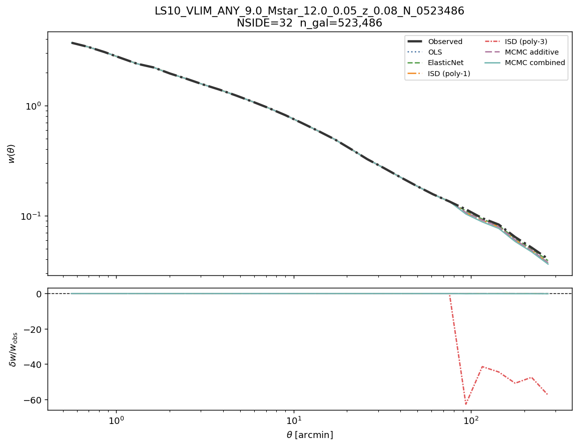
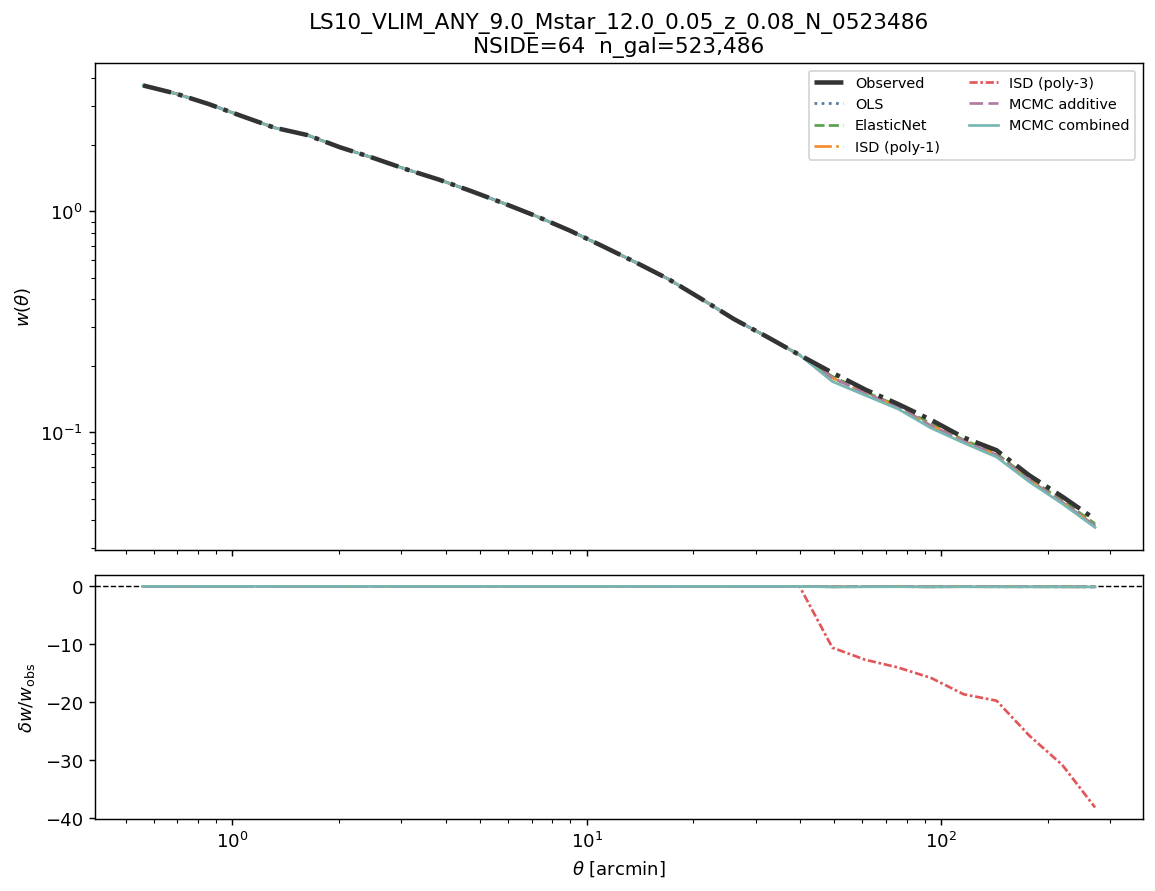
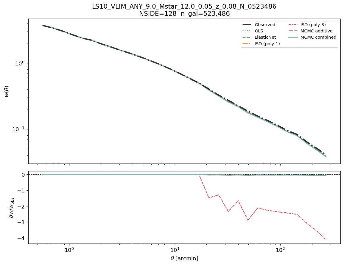
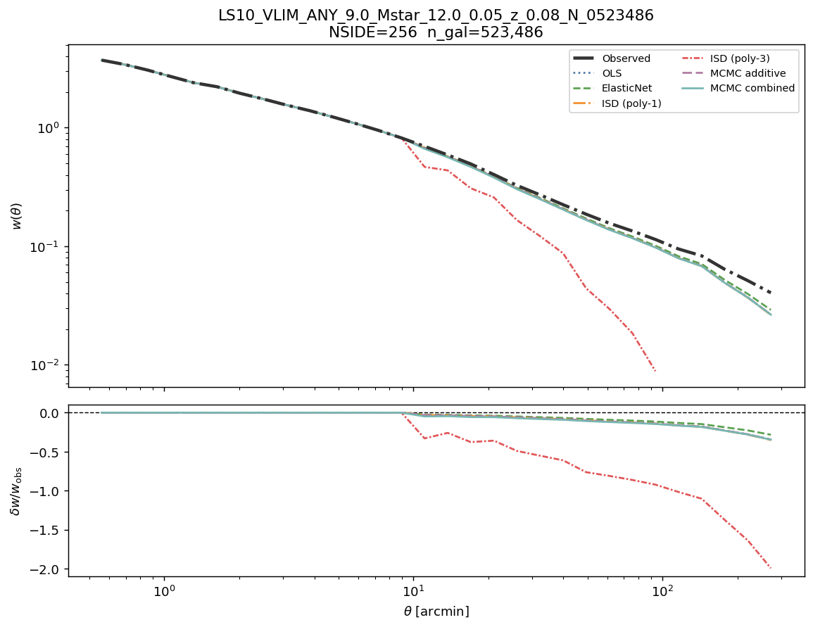
log M* ≥ 9.0, z < 0.08 (N = 523 486)

Systematic weight maps — log M* ≥ 9.0

NSIDE 32 (≈5 600 pix)

NSIDE 64 (≈21 600 pix)

NSIDE 128 (≈84 000 pix)

NSIDE 256 (≈330 000 pix)

Weight distributions — log M* ≥ 9.0

NSIDE 32

NSIDE 64

NSIDE 128

NSIDE 256

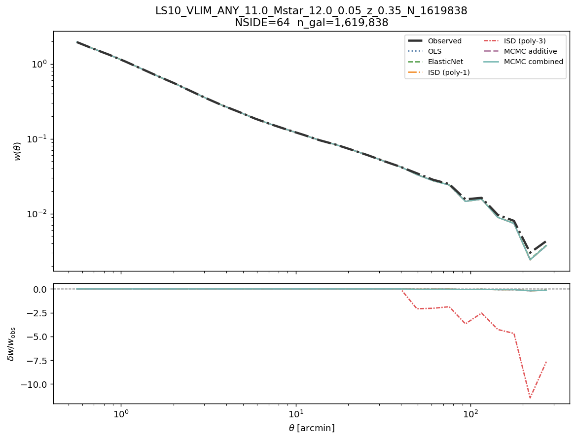
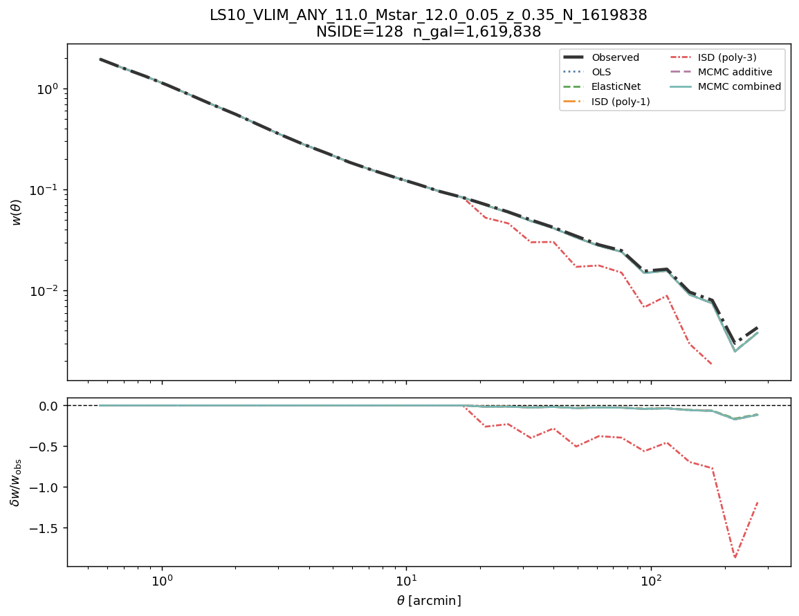
Angular clustering w(θ) — observed and corrected (one line per method) — log M* ≥ 9.0

NSIDE 32

NSIDE 64

NSIDE 128

NSIDE 256

Key numbers — log M* ≥ 9.0

Parameter	NSIDE 32	NSIDE 64	NSIDE 128	NSIDE 256
Ngal	523 486	523 486	523 486	523 486
Npix (good)	5612	21563	84367	324258
LRT λLR (dof=11)	404.2 (Yes)	1489.5 (Yes)	3523.5 (Yes)	7590.4 (Yes)
σ̂ OLS	0.5474	0.6760	0.9909	1.6568
σ̂ ElasticNet	0.5491	0.6768	0.9912	1.6570
σ̂ ISD-1	0.5474	0.6760	0.9910	1.6568
σ̂ ISD-3 ‡	2.9223	3.2810	1.4628	1.7204
σ̂ MCMC-add	0.5483	0.6762	0.9911	1.6568
σ̂ MCMC-comb	0.6736	0.7511	1.0288	1.6008
MCMC-add acc. frac.	0.388	0.390	0.388	0.387
MCMC-comb acc. frac.	0.285	0.296	0.298	0.310
Dominant template	ns_fnt	ns_fnt	ns_fnt	ns_fnt
δw/w at 30′	—	-7.2 %	—	—

‡ ISD-3 uses a degree-3 polynomial expansion and is unreliable at all

resolutions. Do not use ISD-3 weights for any science analysis.

See also

BGS VLIM log M* ≥ 9.0, z < 0.08 — detailed systematic analysis — full template amplitude tables, weight statistics, and cosmological analysis verdict for log M* ≥ 9.0.

log M* ≥ 9.5, z < 0.12 (N = 1 432 502)

Systematic weight maps — log M* ≥ 9.5

NSIDE 32 (≈5 600 pix)

NSIDE 64 (≈21 600 pix)

NSIDE 128 (≈84 000 pix)

NSIDE 256 (≈330 000 pix)

Weight distributions — log M* ≥ 9.5

NSIDE 32

NSIDE 64

NSIDE 128

NSIDE 256

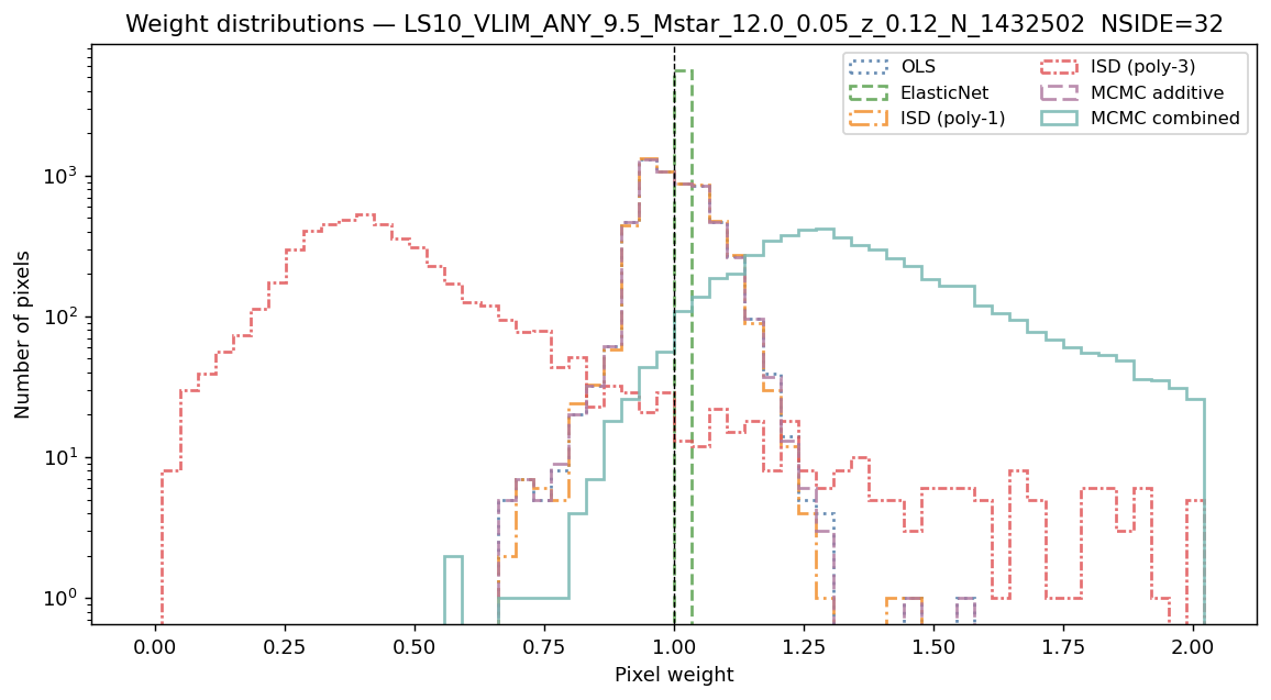
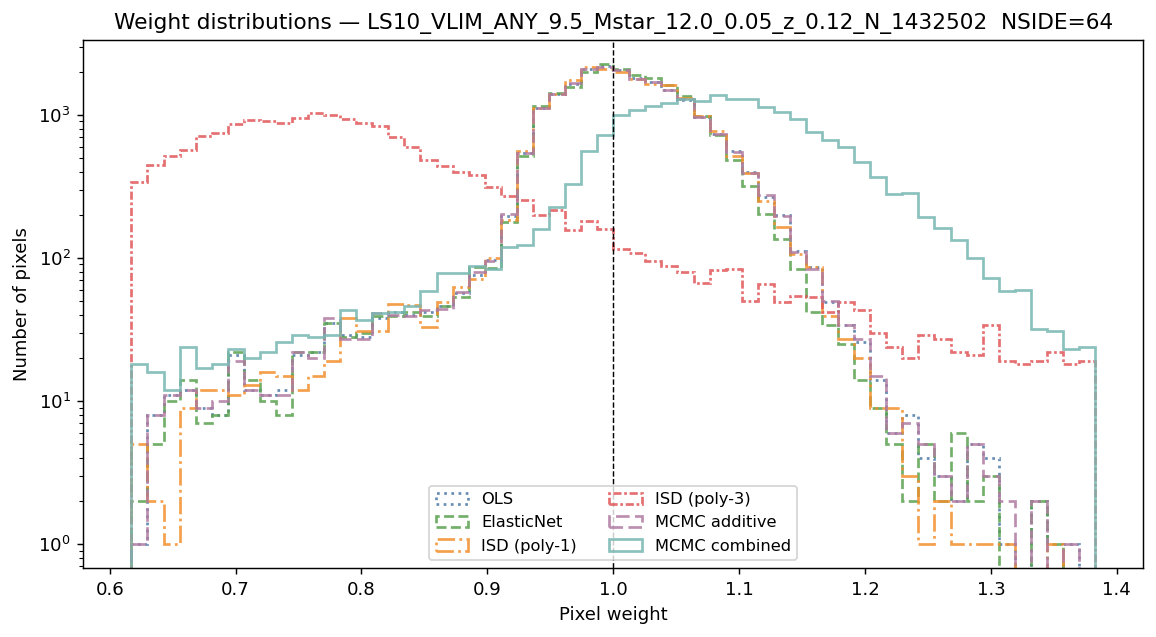
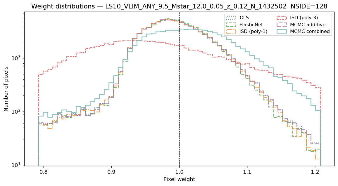
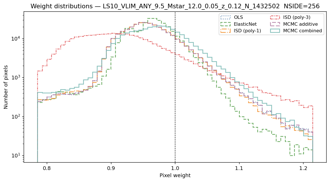
Angular clustering w(θ) — observed and corrected (one line per method) — log M* ≥ 9.5

NSIDE 32

NSIDE 64

NSIDE 128

NSIDE 256

Key numbers — log M* ≥ 9.5

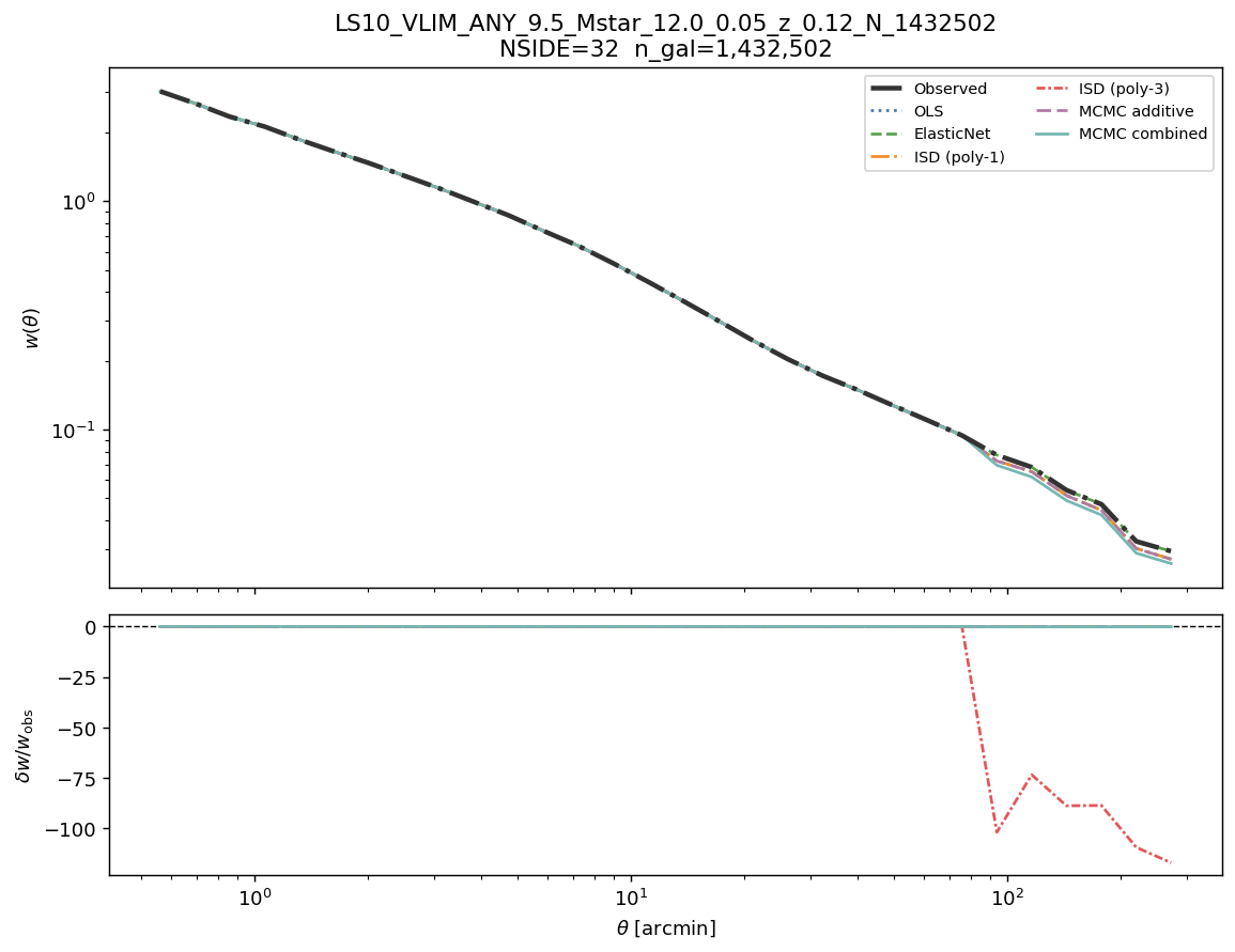
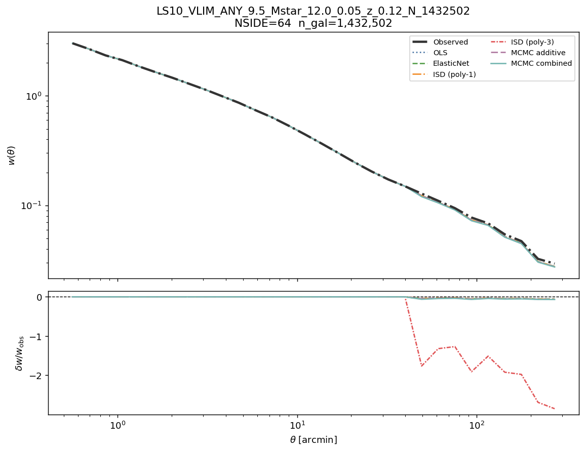
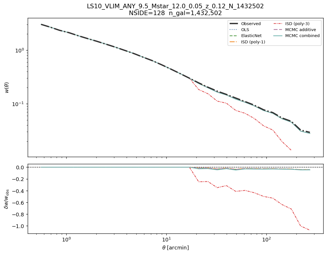
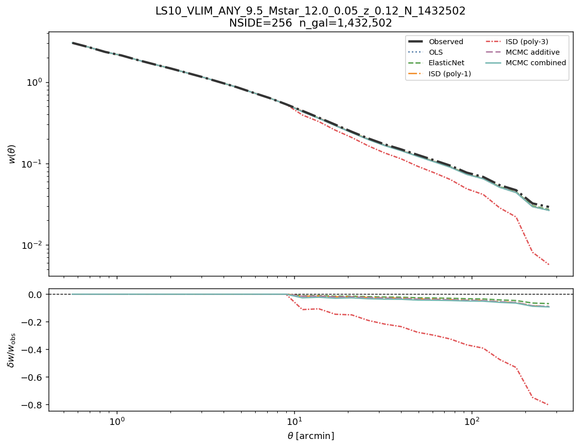
Parameter	NSIDE 32	NSIDE 64	NSIDE 128	NSIDE 256
Ngal	1 432 502	1 432 502	1 432 502	1 432 502
Npix (good)	5611	21637	84627	331787
LRT λLR (dof=11)	621.5 (Yes)	730.6 (Yes)	2267.7 (Yes)	5424.7 (Yes)
σ̂ OLS	0.4708	0.5239	0.7458	1.1021
σ̂ ElasticNet	0.4757	0.5239	0.7458	1.1023
σ̂ ISD-1	0.4708	0.5239	0.7458	1.1022
σ̂ ISD-3 ‡	4.0550	0.7911	0.8344	1.1371
σ̂ MCMC-add	0.4714	0.5240	0.7458	1.1022
σ̂ MCMC-comb	0.6059	0.5545	0.7408	1.0519
MCMC-add acc. frac.	0.387	0.391	0.389	0.388
MCMC-comb acc. frac.	0.288	0.297	0.299	0.296
Dominant template	ns_fnt	ns_fnt	ns_fnt	ns_med
δw/w at 30′	—	-4.8 %	—	—

‡ ISD-3 uses a degree-3 polynomial expansion and is unreliable at all

resolutions. Do not use ISD-3 weights for any science analysis.

See also

BGS VLIM log M* ≥ 9.5, z < 0.12 — detailed systematic analysis — full template amplitude tables, weight statistics, and cosmological analysis verdict for log M* ≥ 9.5.

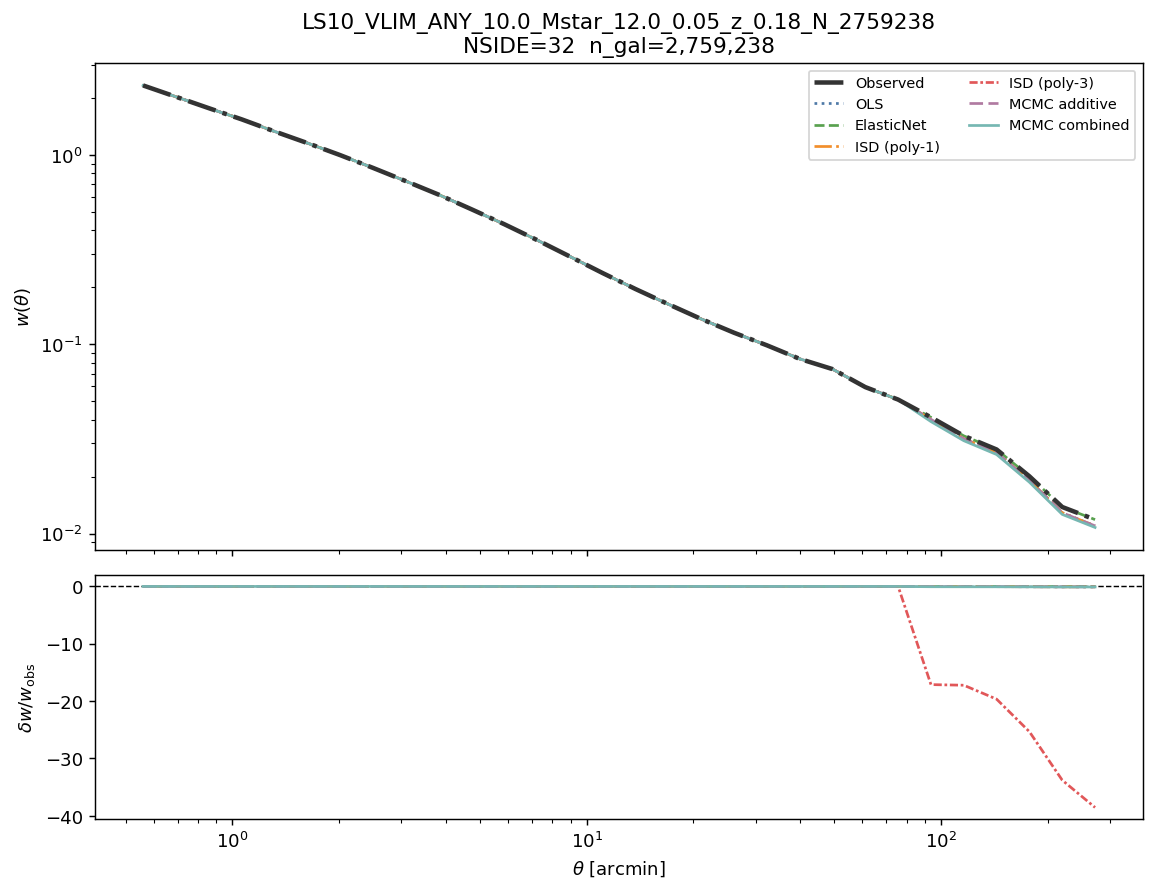
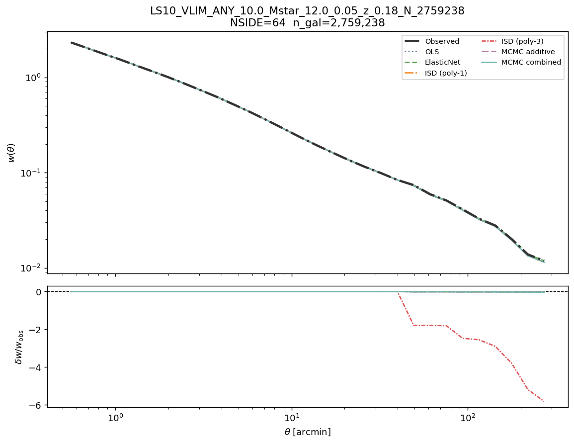
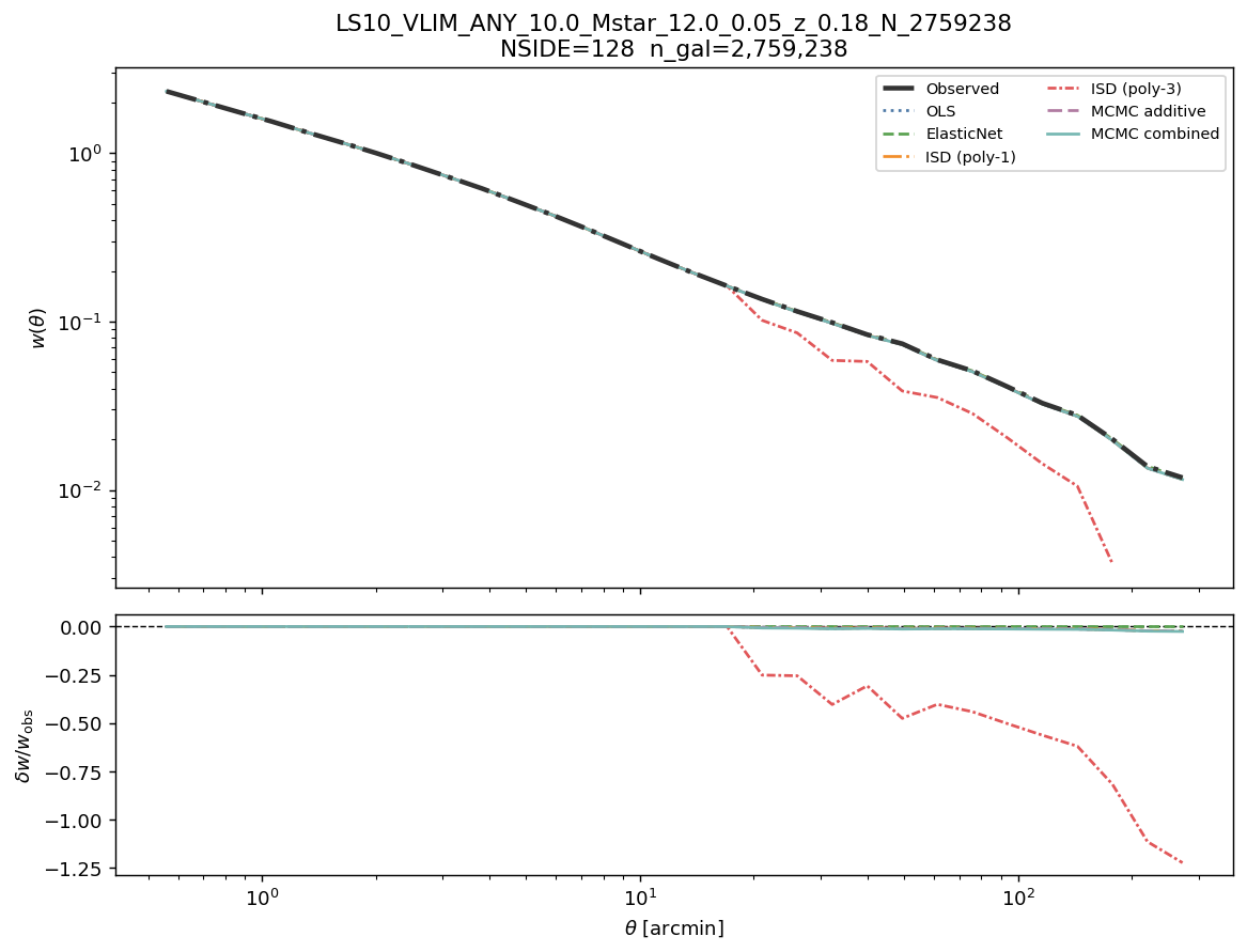
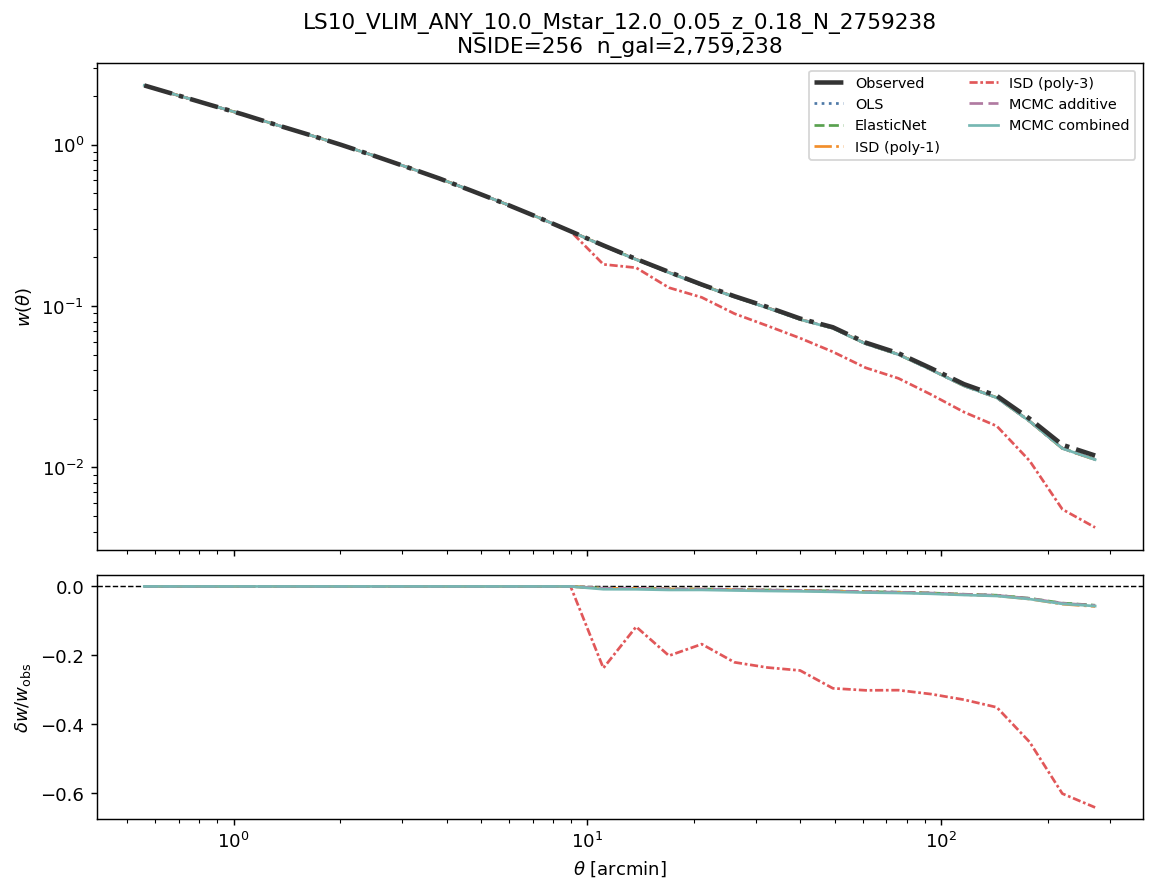
log M* ≥ 10.0, z < 0.18 (N = 2 759 238)

Systematic weight maps — log M* ≥ 10.0

NSIDE 32 (≈5 600 pix)

NSIDE 64 (≈21 600 pix)

NSIDE 128 (≈84 000 pix)

NSIDE 256 (≈330 000 pix)

Weight distributions — log M* ≥ 10.0

NSIDE 32

NSIDE 64

NSIDE 128

NSIDE 256

Angular clustering w(θ) — observed and corrected (one line per method) — log M* ≥ 10.0

NSIDE 32

NSIDE 64

NSIDE 128

NSIDE 256

Key numbers — log M* ≥ 10.0

Parameter	NSIDE 32	NSIDE 64	NSIDE 128	NSIDE 256
Ngal	2 759 238	2 759 238	2 759 238	2 759 238
Npix (good)	5616	21667	84860	332734
LRT λLR (dof=11)	668.9 (Yes)	123.9 (Yes)	324.8 (Yes)	1400.4 (Yes)
σ̂ OLS	0.3801	0.3969	0.5606	0.8173
σ̂ ElasticNet	0.3820	0.3982	0.5616	0.8173
σ̂ ISD-1	0.3801	0.3969	0.5606	0.8173
σ̂ ISD-3 ‡	1.0389	0.7254	0.6472	0.8355
σ̂ MCMC-add	0.3805	0.3969	0.5607	0.8173
σ̂ MCMC-comb	0.4224	0.3817	0.5337	0.7855
MCMC-add acc. frac.	0.386	0.389	0.388	0.386
MCMC-comb acc. frac.	0.281	0.277	0.288	0.306
Dominant template	ns_fnt	ns_fnt	ns_fnt	ns_med
δw/w at 30′	—	-0.4 %	—	—

‡ ISD-3 uses a degree-3 polynomial expansion and is unreliable at all

resolutions. Do not use ISD-3 weights for any science analysis.

See also

BGS VLIM log M* ≥ 10.0, z < 0.18 — detailed systematic analysis — full template amplitude tables, weight statistics, and cosmological analysis verdict for log M* ≥ 10.0.

log M* ≥ 10.25, z < 0.22 (N = 3 308 841)

Systematic weight maps — log M* ≥ 10.25

NSIDE 32 (≈5 600 pix)

NSIDE 64 (≈21 600 pix)

NSIDE 128 (≈84 000 pix)

NSIDE 256 (≈330 000 pix)

Weight distributions — log M* ≥ 10.25

NSIDE 32

NSIDE 64

NSIDE 128

NSIDE 256

Angular clustering w(θ) — observed and corrected (one line per method) — log M* ≥ 10.25

NSIDE 32

NSIDE 64

NSIDE 128

NSIDE 256

Key numbers — log M* ≥ 10.25

Parameter	NSIDE 32	NSIDE 64	NSIDE 128	NSIDE 256
Ngal	3 308 841	3 308 841	3 308 841	3 308 841
Npix (good)	5618	21669	84831	333050
LRT λLR (dof=11)	808.3 (Yes)	66.9 (Yes)	206.8 (Yes)	740.9 (Yes)
σ̂ OLS	0.3417	0.3434	0.4900	0.7212
σ̂ ElasticNet	0.3436	0.3434	0.4900	0.7212
σ̂ ISD-1	0.3417	0.3434	0.4900	0.7212
σ̂ ISD-3 ‡	0.8803	0.9979	0.5192	0.7267
σ̂ MCMC-add	0.3421	0.3435	0.4900	0.7212
σ̂ MCMC-comb	0.3903	0.3343	0.4739	0.6964
MCMC-add acc. frac.	0.387	0.389	0.388	0.388
MCMC-comb acc. frac.	0.280	0.277	0.288	0.298
Dominant template	ns_fnt	ns_fnt	ns_fnt	ns_med
δw/w at 30′	—	n/a	—	—

‡ ISD-3 uses a degree-3 polynomial expansion and is unreliable at all

resolutions. Do not use ISD-3 weights for any science analysis.

See also

BGS VLIM log M* ≥ 10.25, z < 0.22 — detailed systematic analysis — full template amplitude tables, weight statistics, and cosmological analysis verdict for log M* ≥ 10.25.

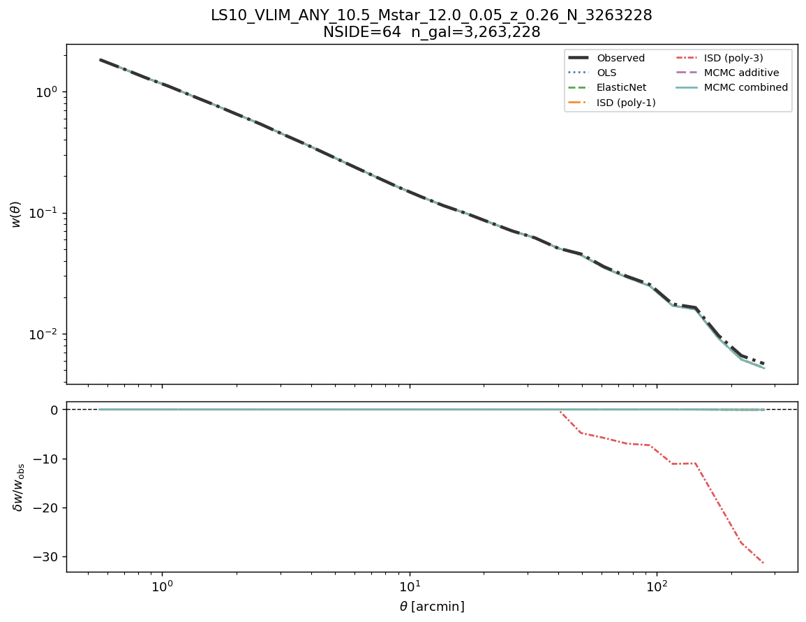
log M* ≥ 10.5, z < 0.26 (N = 3 263 228)

Systematic weight maps — log M* ≥ 10.5

NSIDE 32 (≈5 600 pix)

NSIDE 64 (≈21 600 pix)

NSIDE 128 (≈84 000 pix)

NSIDE 256 (≈330 000 pix)

Weight distributions — log M* ≥ 10.5

NSIDE 32

NSIDE 64

NSIDE 128

NSIDE 256

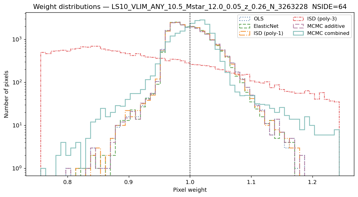
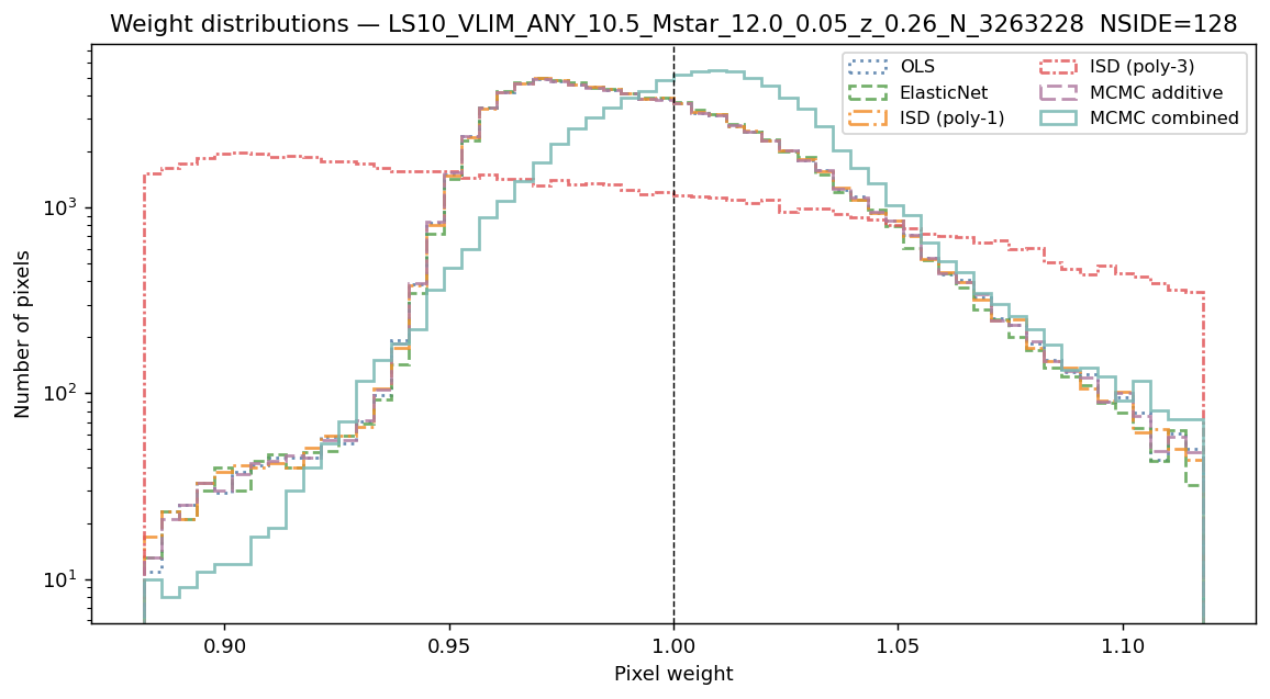
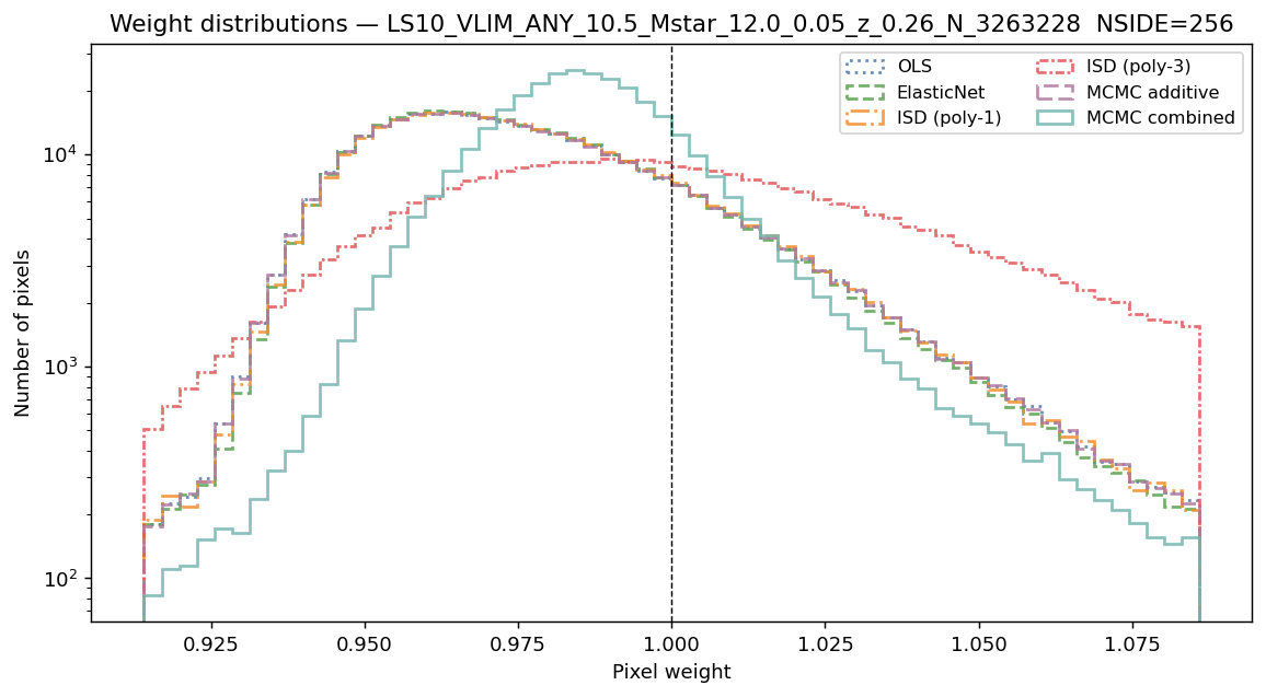
Angular clustering w(θ) — observed and corrected (one line per method) — log M* ≥ 10.5

NSIDE 32

NSIDE 64

NSIDE 128

NSIDE 256

Key numbers — log M* ≥ 10.5

Parameter	NSIDE 32	NSIDE 64	NSIDE 128	NSIDE 256
Ngal	3 263 228	3 263 228	3 263 228	3 263 228
Npix (good)	5617	21675	84811	332982
LRT λLR (dof=11)	952.9 (Yes)	69.6 (Yes)	233.9 (Yes)	557.4 (Yes)
σ̂ OLS	0.3238	0.3089	0.4477	0.6676
σ̂ ElasticNet	0.3252	0.3089	0.4477	0.6676
σ̂ ISD-1	0.3238	0.3089	0.4477	0.6677
σ̂ ISD-3 ‡	0.6415	1.0787	0.5027	0.6727
σ̂ MCMC-add	0.3241	0.3089	0.4478	0.6677
σ̂ MCMC-comb	0.3731	0.3104	0.4514	0.6593
MCMC-add acc. frac.	0.388	0.390	0.389	0.388
MCMC-comb acc. frac.	0.282	0.287	0.288	0.298
Dominant template	ns_fnt	ns_fnt	ns_fnt	ns_med
δw/w at 30′	—	n/a	—	—

‡ ISD-3 uses a degree-3 polynomial expansion and is unreliable at all

resolutions. Do not use ISD-3 weights for any science analysis.

See also

BGS VLIM log M* ≥ 10.5, z < 0.26 — detailed systematic analysis — full template amplitude tables, weight statistics, and cosmological analysis verdict for log M* ≥ 10.5.

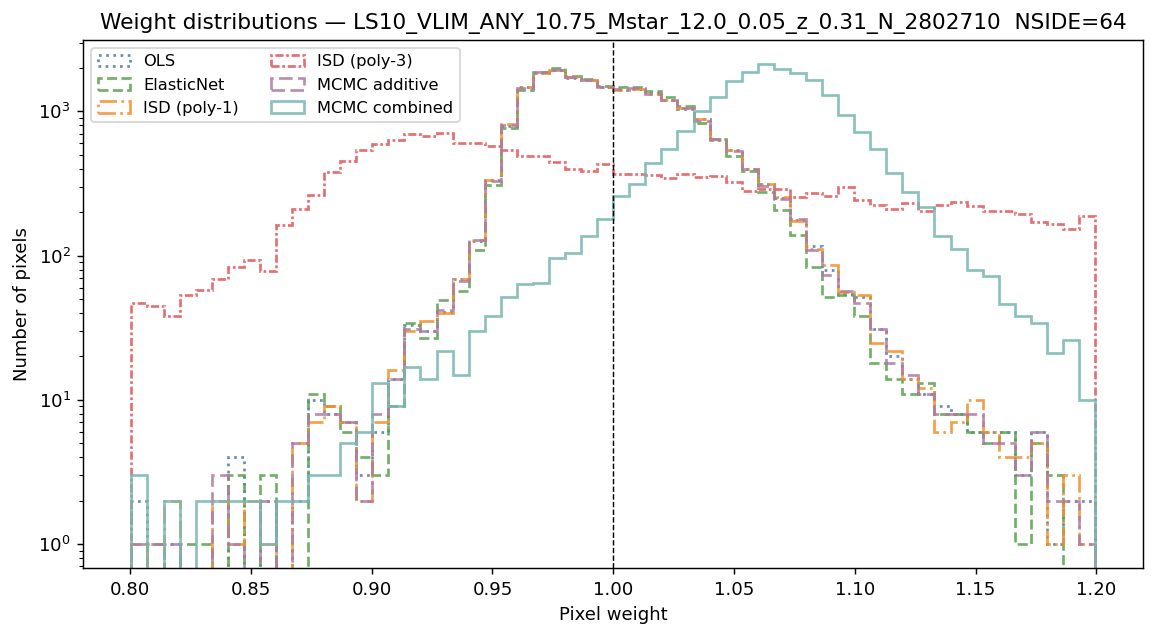
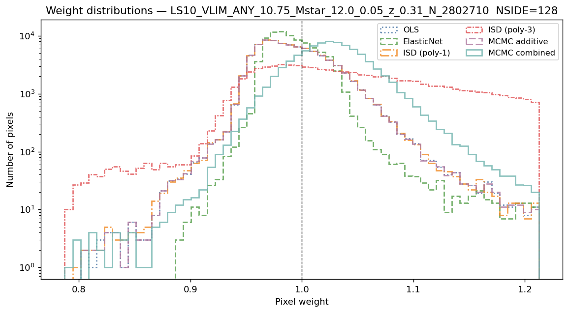
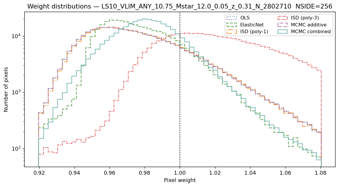
log M* ≥ 10.75, z < 0.31 (N = 2 802 710)

Systematic weight maps — log M* ≥ 10.75

NSIDE 32 (≈5 600 pix)

NSIDE 64 (≈21 600 pix)

NSIDE 128 (≈84 000 pix)

NSIDE 256 (≈330 000 pix)

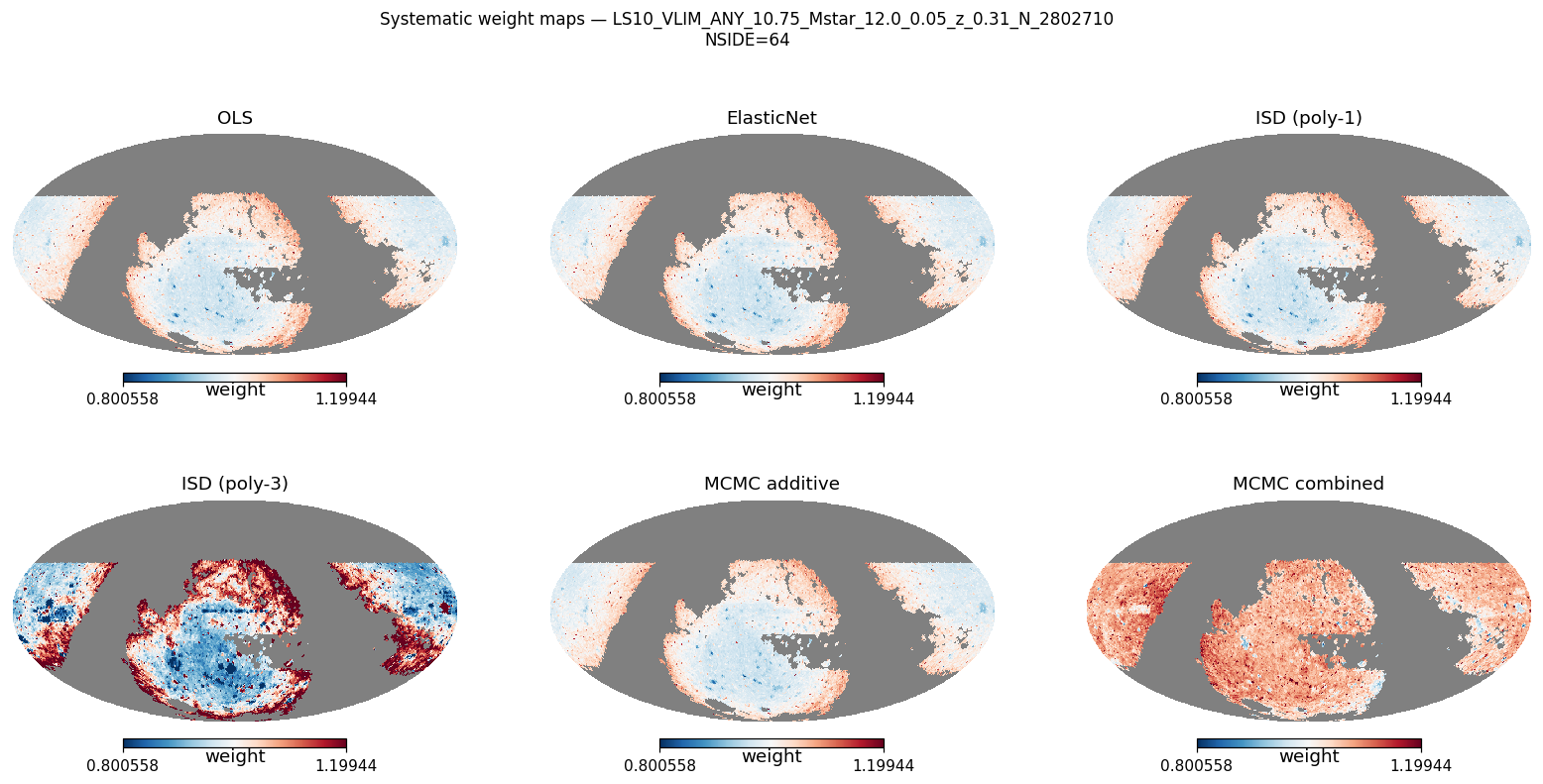
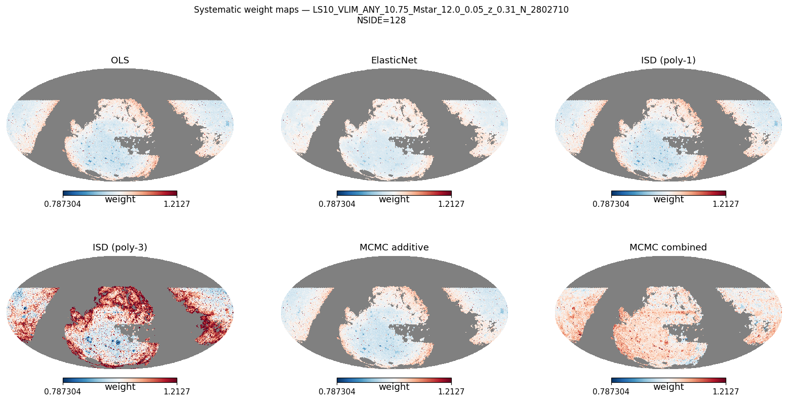
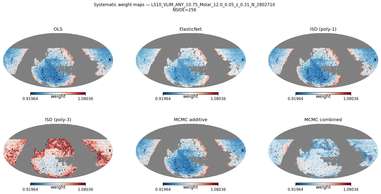
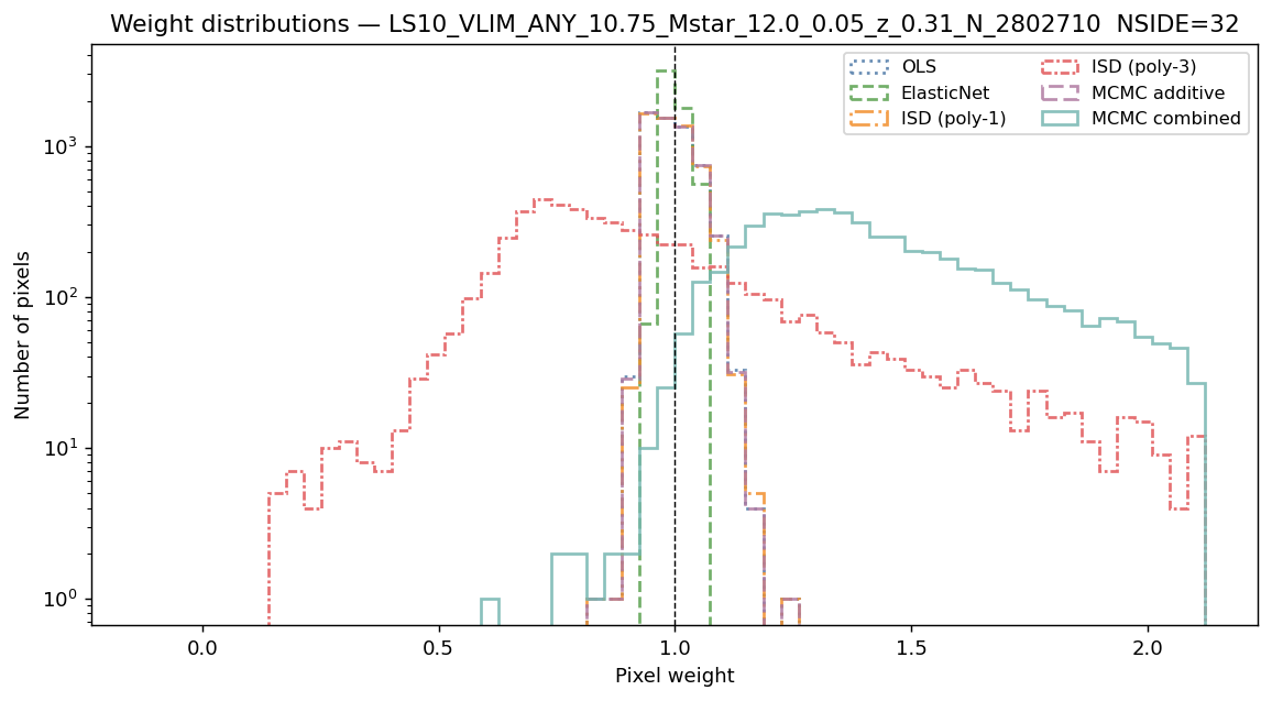
Weight distributions — log M* ≥ 10.75

NSIDE 32

NSIDE 64

NSIDE 128

NSIDE 256

Angular clustering w(θ) — observed and corrected (one line per method) — log M* ≥ 10.75

NSIDE 32

NSIDE 64

NSIDE 128

NSIDE 256

Key numbers — log M* ≥ 10.75

Parameter	NSIDE 32	NSIDE 64	NSIDE 128	NSIDE 256
Ngal	2 802 710	2 802 710	2 802 710	2 802 710
Npix (good)	5618	21662	84824	332812
LRT λLR (dof=11)	1169.2 (Yes)	89.1 (Yes)	287.4 (Yes)	580.6 (Yes)
σ̂ OLS	0.3057	0.2831	0.4190	0.6422
σ̂ ElasticNet	0.3069	0.2831	0.4194	0.6423
σ̂ ISD-1	0.3057	0.2831	0.4190	0.6422
σ̂ ISD-3 ‡	0.6315	0.4658	0.9265	0.6894
σ̂ MCMC-add	0.3061	0.2831	0.4191	0.6422
σ̂ MCMC-comb	0.3982	0.3009	0.4300	0.6305
MCMC-add acc. frac.	0.388	0.392	0.388	0.388
MCMC-comb acc. frac.	0.295	0.281	0.293	0.297
Dominant template	ns_fnt	ns_fnt	ns_fnt	ns_med
δw/w at 30′	—	n/a	—	—

‡ ISD-3 uses a degree-3 polynomial expansion and is unreliable at all

resolutions. Do not use ISD-3 weights for any science analysis.

See also

BGS VLIM log M* ≥ 10.75, z < 0.31 — detailed systematic analysis — full template amplitude tables, weight statistics, and cosmological analysis verdict for log M* ≥ 10.75.

log M* ≥ 11.0, z < 0.35 (N = 1 619 838)

Systematic weight maps — log M* ≥ 11.0

NSIDE 32 (≈5 600 pix)

NSIDE 64 (≈21 600 pix)

NSIDE 128 (≈84 000 pix)

NSIDE 256 (≈330 000 pix)

Weight distributions — log M* ≥ 11.0

NSIDE 32

NSIDE 64

NSIDE 128

NSIDE 256

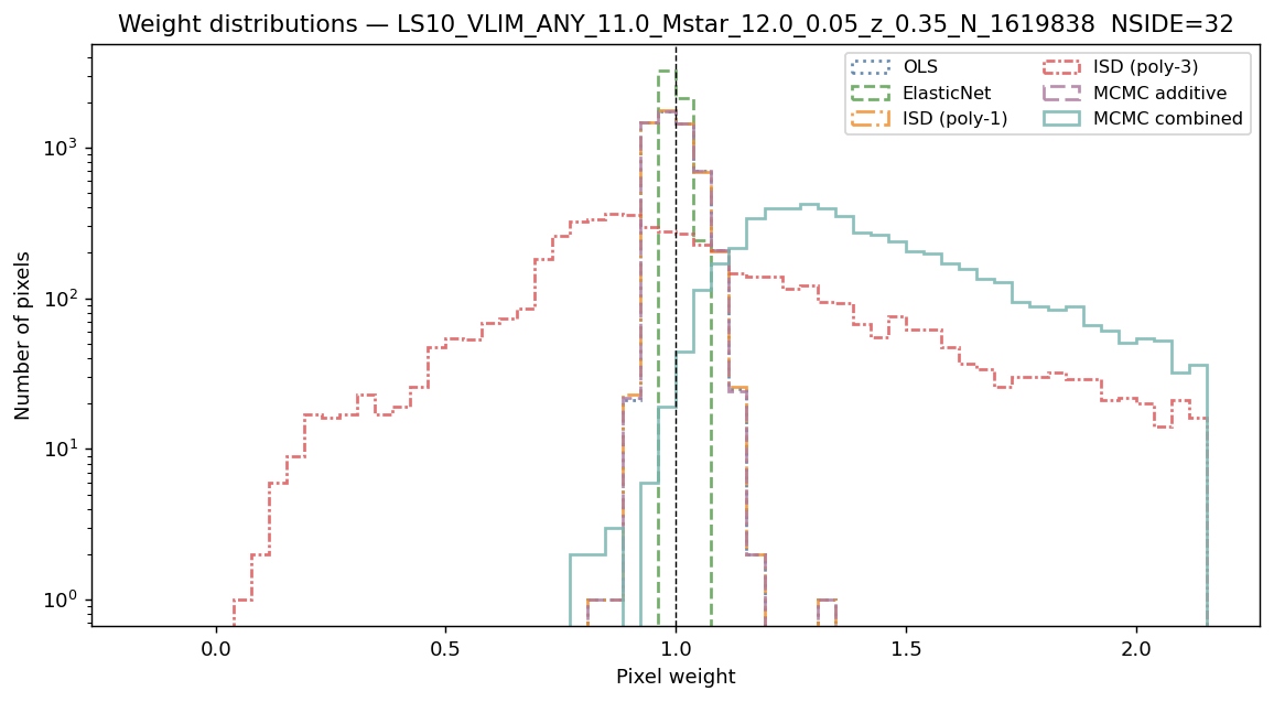
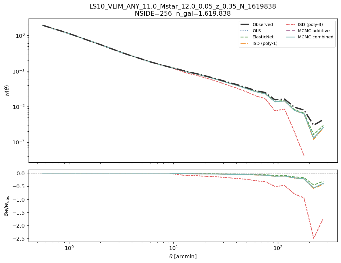
Angular clustering w(θ) — observed and corrected (one line per method) — log M* ≥ 11.0

NSIDE 32

NSIDE 64

NSIDE 128

NSIDE 256

Key numbers — log M* ≥ 11.0

Parameter	NSIDE 32	NSIDE 64	NSIDE 128	NSIDE 256
Ngal	1 619 838	1 619 838	1 619 838	1 619 838
Npix (good)	5614	21646	84719	332484
LRT λLR (dof=11)	997.4 (Yes)	75.1 (Yes)	206.1 (Yes)	682.0 (Yes)
σ̂ OLS	0.2971	0.2974	0.4580	0.7557
σ̂ ElasticNet	0.2985	0.2974	0.4580	0.7558
σ̂ ISD-1	0.2971	0.2974	0.4580	0.7558
σ̂ ISD-3 ‡	0.7040	0.4975	0.4899	0.7786
σ̂ MCMC-add	0.2974	0.2975	0.4580	0.7558
σ̂ MCMC-comb	0.3927	0.3052	0.4716	0.7256
MCMC-add acc. frac.	0.389	0.390	0.389	0.388
MCMC-comb acc. frac.	0.292	0.289	0.291	0.288
Dominant template	ns_fnt	ns_fnt	ns_fnt	ns_med
δw/w at 30′	—	-0.1 %	—	—

‡ ISD-3 uses a degree-3 polynomial expansion and is unreliable at all

resolutions. Do not use ISD-3 weights for any science analysis.

See also

BGS VLIM log M* ≥ 11.0, z < 0.35 — detailed systematic analysis — full template amplitude tables, weight statistics, and cosmological analysis verdict for log M* ≥ 11.0.

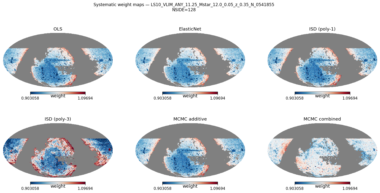
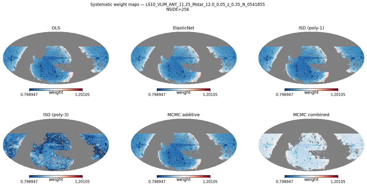
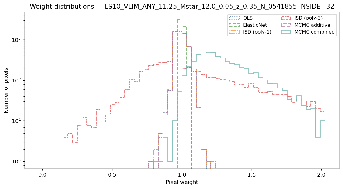
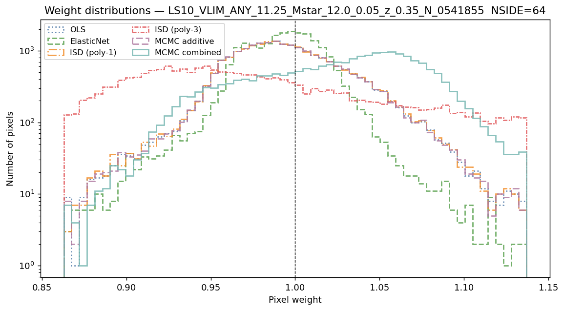
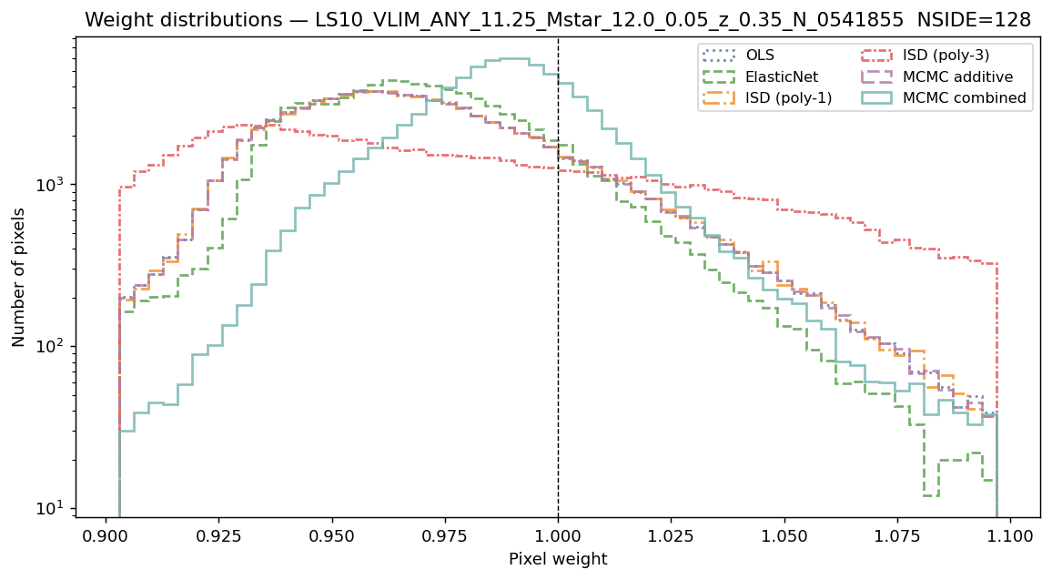
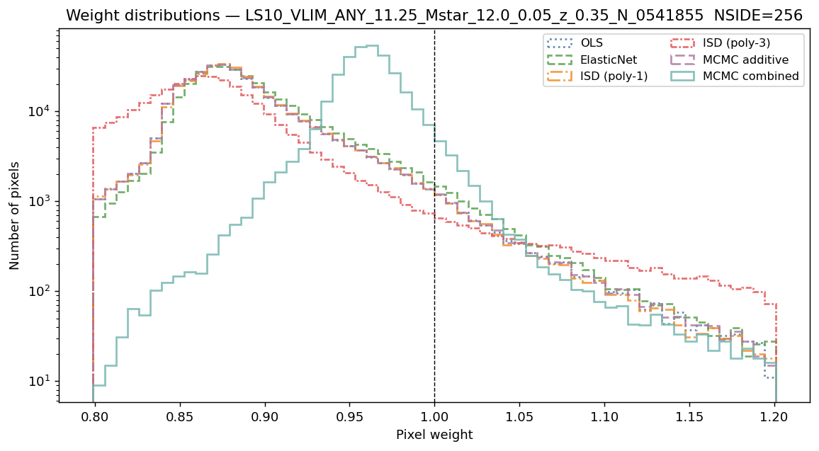
log M* ≥ 11.25, z < 0.35 (N = 541 855)

Systematic weight maps — log M* ≥ 11.25

NSIDE 32 (≈5 600 pix)

NSIDE 64 (≈21 600 pix)

NSIDE 128 (≈84 000 pix)

NSIDE 256 (≈330 000 pix)

Weight distributions — log M* ≥ 11.25

NSIDE 32

NSIDE 64

NSIDE 128

NSIDE 256

Angular clustering w(θ) — observed and corrected (one line per method) — log M* ≥ 11.25

NSIDE 32

NSIDE 64

NSIDE 128

NSIDE 256

Key numbers — log M* ≥ 11.25

Parameter	NSIDE 32	NSIDE 64	NSIDE 128	NSIDE 256
Ngal	541 855	541 855	541 855	541 855
Npix (good)	5609	21555	84131	325324
LRT λLR (dof=11)	613.5 (Yes)	123.4 (Yes)	140.8 (Yes)	597.3 (Yes)
σ̂ OLS	0.3308	0.3842	0.6405	1.2602
σ̂ ElasticNet	0.3319	0.3846	0.6406	1.2603
σ̂ ISD-1	0.3308	0.3842	0.6405	1.2602
σ̂ ISD-3 ‡	0.7031	0.6196	0.6454	1.3131
σ̂ MCMC-add	0.3313	0.3843	0.6406	1.2602
σ̂ MCMC-comb	0.4062	0.3930	0.6329	1.2117
MCMC-add acc. frac.	0.386	0.389	0.387	0.390
MCMC-comb acc. frac.	0.293	0.288	0.287	0.301
Dominant template	ns_fnt	ns_fnt	ns_med	ns_fnt
δw/w at 30′	—	+2.2 %	—	—

‡ ISD-3 uses a degree-3 polynomial expansion and is unreliable at all

resolutions. Do not use ISD-3 weights for any science analysis.

See also

BGS VLIM log M* ≥ 11.25, z < 0.35 — detailed systematic analysis — full template amplitude tables, weight statistics, and cosmological analysis verdict for log M* ≥ 11.25.

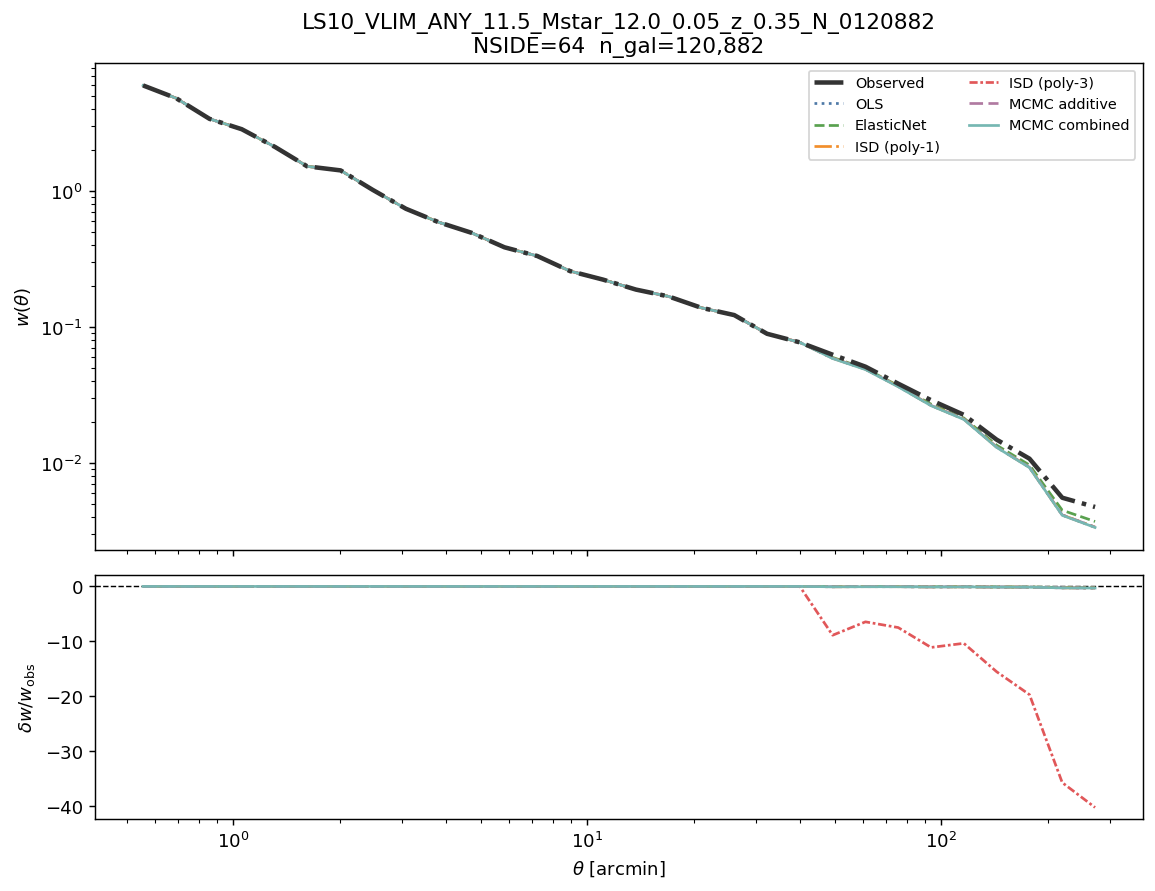
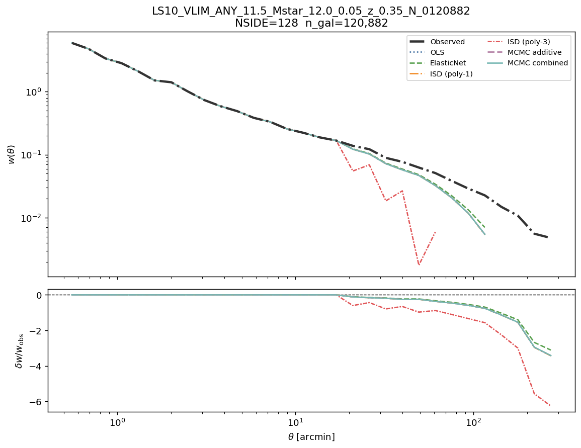
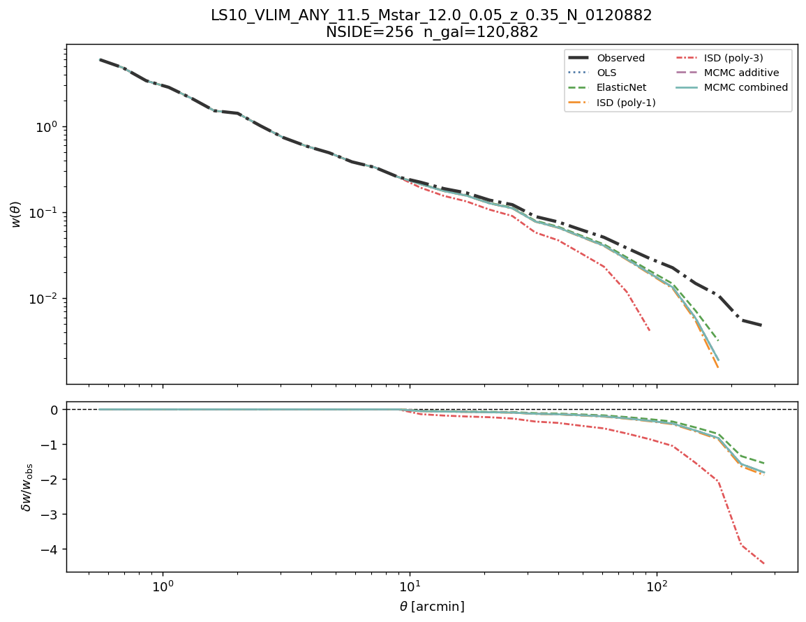
log M* ≥ 11.5, z < 0.35 (N = 120 882)

Systematic weight maps — log M* ≥ 11.5

NSIDE 32 (≈5 600 pix)

NSIDE 64 (≈21 600 pix)

NSIDE 128 (≈84 000 pix)

NSIDE 256 (≈330 000 pix)

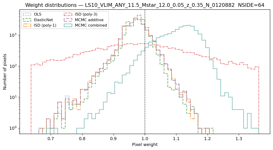
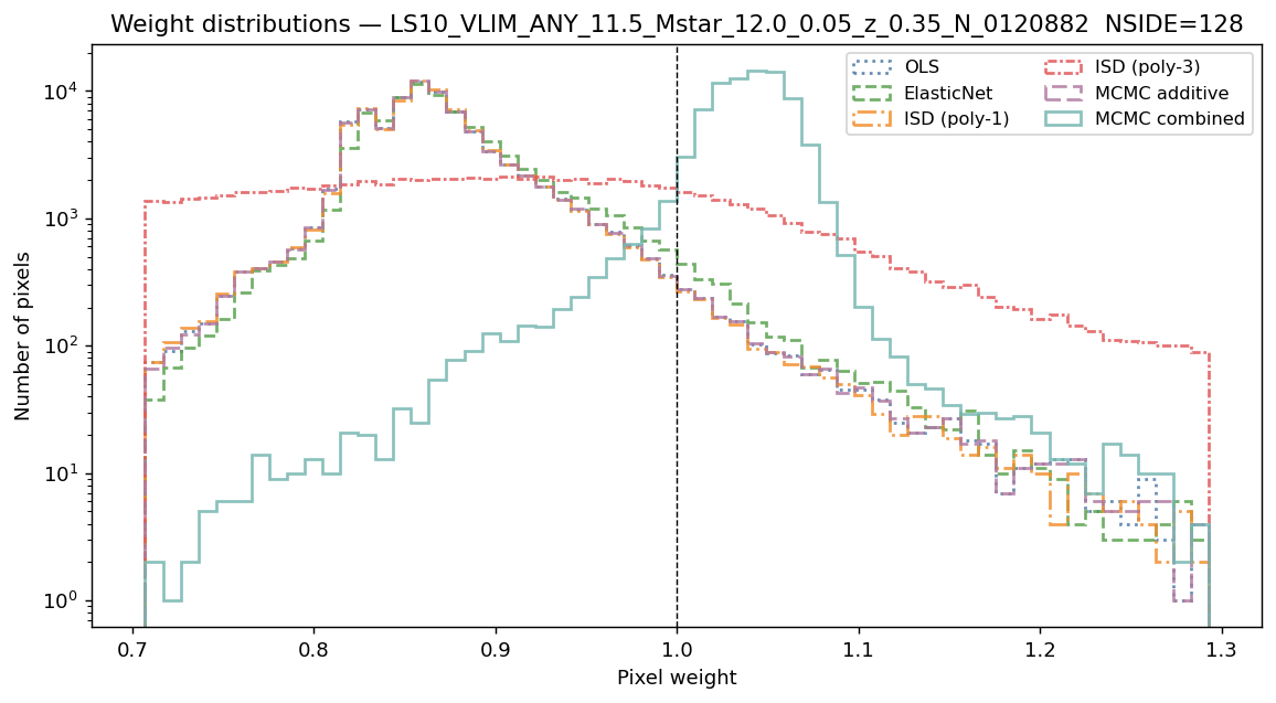
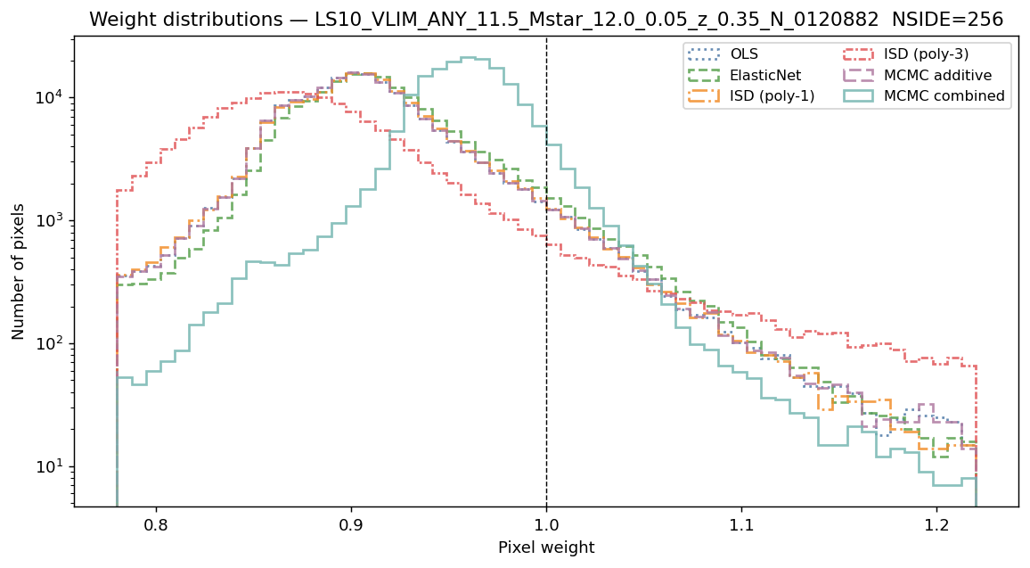
Weight distributions — log M* ≥ 11.5

NSIDE 32

NSIDE 64

NSIDE 128

NSIDE 256

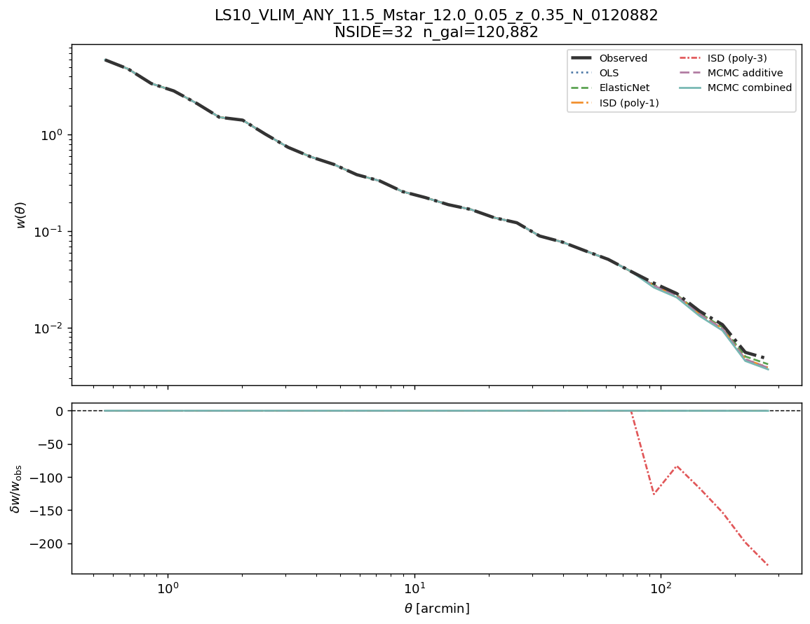
Angular clustering w(θ) — observed and corrected (one line per method) — log M* ≥ 11.5

NSIDE 32

NSIDE 64

NSIDE 128

NSIDE 256

Key numbers — log M* ≥ 11.5

Parameter	NSIDE 32	NSIDE 64	NSIDE 128	NSIDE 256
Ngal	120 882	120 882	120 882	120 882
Npix (good)	5571	21344	83244	180102
LRT λLR (dof=11)	352.1 (Yes)	151.5 (Yes)	196.7 (Yes)	575.1 (Yes)
σ̂ OLS	0.4451	0.6438	1.3802	2.1098
σ̂ ElasticNet	0.4453	0.6440	1.3803	2.1098
σ̂ ISD-1	0.4451	0.6438	1.3802	2.1098
σ̂ ISD-3 ‡	2.1206	1.0507	1.4249	2.1189
σ̂ MCMC-add	0.4455	0.6441	1.3803	2.1098
σ̂ MCMC-comb	0.5862	0.7104	1.4304	2.0211
MCMC-add acc. frac.	0.387	0.388	0.388	0.387
MCMC-comb acc. frac.	0.281	0.287	0.297	0.283
Dominant template	ns_fnt	ns_med	ns_fnt	ns_fnt
δw/w at 30′	—	+0.7 %	—	—

‡ ISD-3 uses a degree-3 polynomial expansion and is unreliable at all

resolutions. Do not use ISD-3 weights for any science analysis.

See also

BGS VLIM log M* ≥ 11.5, z < 0.35 — detailed systematic analysis — full template amplitude tables, weight statistics, and cosmological analysis verdict for log M* ≥ 11.5.

---

MAP parameters — 11-template analysis (NSIDE 64)

The table below lists MAP estimates from the NSIDE = 64 run (11 templates). Column abbreviations:

Abbreviation	Full template name
EBV	LS10:EBV
GD_G	LS10:GALDEPTH_G
GD_R	LS10:GALDEPTH_R
GD_Z	LS10:GALDEPTH_Z
NOBS_R	LS10:NOBS_R
PSF_R	LS10:PSFSIZE_R
ns_fnt	GAIA:nstar_faint
ns_med	GAIA:nstar_medium
bp_fl	GAIA:phot_bp_mean_flux
g_fl	GAIA:phot_g_mean_flux
rp_fl	GAIA:phot_rp_mean_flux

The dominant systematic in all samples is GAIA:nstar_faint (stellar density).

Additive MAP parameters \(\hat{a}_i\) (MCMC-add, NSIDE 64)

Sample (log M* ≥, z <)	EBV	GD_G	GD_R	GD_Z	NOBS_R	PSF_R	ns_fnt	ns_med	bp_fl	g_fl	rp_fl
9.0, 0.08	+0.4449	-0.3143	-0.0246	+0.0372	-0.0339	-0.0211	-0.0266	+0.0826	+0.0002	-0.0040	-0.0086
9.5, 0.12	+0.5516	-0.3989	-0.0201	+0.0142	-0.0119	-0.0158	-0.0233	+0.0724	+0.0017	-0.0113	+0.0116
10.0, 0.18	+0.3631	-0.2667	-0.0029	+0.0037	-0.0165	+0.0036	-0.0138	+0.0296	+0.0066	-0.0158	-0.0059
10.25, 0.22	+0.3181	-0.2279	-0.0050	+0.0116	-0.0253	-0.0021	-0.0087	+0.0188	+0.0042	-0.0112	-0.0098
10.5, 0.26	+0.3550	-0.2488	-0.0138	+0.0288	-0.0394	-0.0101	-0.0061	+0.0143	+0.0025	-0.0069	-0.0043
10.75, 0.31	+0.3222	-0.2216	-0.0149	+0.0290	-0.0415	-0.0122	+0.0017	+0.0076	+0.0045	-0.0023	-0.0047
11.0, 0.35	+0.3608	-0.2525	-0.0174	+0.0316	-0.0427	-0.0060	+0.0067	+0.0046	+0.0055	+0.0011	-0.0067
11.25, 0.35	+0.2755	-0.1944	-0.0334	+0.0530	-0.0511	-0.0029	+0.0132	+0.0034	+0.0054	+0.0044	-0.0079
11.5, 0.35	+0.0901	-0.1024	-0.0288	+0.0501	-0.0527	+0.0031	+0.0193	+0.0065	+0.0083	+0.0073	-0.0098

Multiplicative MAP parameters \(\hat{b}_i\) (MCMC-comb, NSIDE 64)

Sample (log M* ≥, z <)	EBV	GD_G	GD_R	GD_Z	NOBS_R	PSF_R	ns_fnt	ns_med	bp_fl	g_fl	rp_fl
9.0, 0.08	+1.1908	-0.6523	-0.0060	+0.0280	-0.0428	+0.0069	-0.0181	+0.1162	+0.0850	-0.0147	+0.0194
9.5, 0.12	+0.9926	-0.6066	-0.0135	+0.0111	-0.0257	-0.0075	-0.0153	+0.0965	+0.0415	-0.0176	+0.0417
10.0, 0.18	+0.1685	-0.1994	-0.0108	-0.0167	+0.0121	+0.0301	-0.0256	+0.0540	+0.0002	-0.0089	+0.0098
10.25, 0.22	-0.0279	-0.0258	+0.0163	-0.0162	-0.0133	+0.0322	-0.0187	+0.0358	-0.0066	-0.0026	-0.0009
10.5, 0.26	+0.1317	-0.0659	+0.0100	+0.0120	-0.0546	+0.0254	-0.0166	+0.0227	-0.0045	+0.0119	+0.0044
10.75, 0.31	+0.6170	-0.3227	-0.0108	+0.0250	-0.0498	+0.0117	-0.0050	+0.0109	-0.0076	+0.0166	+0.0129
11.0, 0.35	+0.3700	-0.2100	-0.0251	+0.0332	-0.0359	+0.0297	+0.0049	+0.0139	-0.0026	+0.0101	+0.0044
11.25, 0.35	+0.3944	-0.2422	-0.0343	+0.0288	-0.0168	+0.0513	+0.0137	+0.0098	-0.0063	+0.0054	-0.0016
11.5, 0.35	+0.6752	-0.3323	-0.0356	+0.0188	+0.0143	+0.0415	+0.0077	+0.0134	+0.0047	+0.0119	-0.0027

Key pattern: GAIA:nstar_faint (ns_fnt) carries the largest amplitude in nearly every sample. The anti-correlated GAIA:nstar_medium (ns_med) reflects stellar colour selection at moderate magnitudes. LS10:GALDEPTH_R captures imaging-depth variations in the \(r\) band.

---

Outcome

The systematic decontamination analysis of LS10 BGS VLIM (\(r < 19.5\)) yields a clear conclusion:

• Systematics are present and detectable. The LRT rejects the additive null for all nine samples at all four NSIDEs (dof = 11, \(\chi^2_{11,\,0.95} \approx 19.7\)). The dominant source is GAIA stellar density (nstar_faint).

• Sub-degree clustering is safe after correction. At \(\theta < 30'\), the fractional correction is \(\delta w/w < 2\%\) for log M* ≥ 10.0.

• Large-angle clustering requires the correction. At \(\theta > 2°\), stellar contamination contributes 10–40 % to \(w(\theta)\).

• Use NSIDE 64 weights for all science. NSIDE 32 overfits the multiplicative model (too few pixels). NSIDE 128/256 add noise without improving the fit.

• Recommended weight: WEIGHT_COMB (NSIDE 64) for all science.