Model test matrix
This page reports the results of a comprehensive two-tier test battery that evaluates all six implemented methods across every combination of additive and multiplicative contamination configurations. The key diagnostic is the ratio
computed at every unmasked pixel \(p\). A perfect correction gives \(\mathcal{R} = 1\) everywhere; the standard deviation \(\sigma[\mathcal{R}]\) quantifies residual contamination after correction (lower is better; the irreducible floor is set by Poisson shot noise).
Configuration
Parameter |
Value |
|---|---|
NSIDE |
32 (pixel area ≈ 3.4 deg², ~8 000 pixels in footprint) |
Galactic footprint |
\(|b_{\rm gal}| > 20°\) (≈ 66 % of sky) |
Mean galaxies per pixel \(\bar{n}\) |
50 |
Random / galaxy ratio |
8× |
Lognormal field width \(\sigma_G\) |
0.5 |
Injected amplitude \(|a_i^{\rm true}|\) and \(|b_i^{\rm true}|\) |
0.10 per active template |
MCMC walkers / steps / burn-in |
100 / 600 / 100 |
Script |
|
Output |
|
Template set
Seven synthetic HEALPix templates are used throughout:
Label |
Family |
Power spectrum / description |
|---|---|---|
synth_0 |
0, seed 0 |
\(C_\ell \propto e^{-\ell/500}\) — large-scale coherent artefact |
synth_1 |
1, seed 0 |
\(C_\ell \propto e^{-(\ell/250)^2}\) — intermediate-scale artefact |
synth_2 |
2, seed 0 |
\(C_\ell \propto (\ell+1)^{-2}\) — steep power law |
synth_3 |
3, seed 0 |
\(C_\ell \propto (\ell+1)^{-1}\) — shallow power law |
synth_4 |
4, seed 0 |
\(C_\ell = {\rm const}\) — white noise |
synth_5 |
0, seed 5 |
\(C_\ell \propto e^{-\ell/500}\) — second large-scale map (GAIA stand-in) |
synth_6 |
2, seed 5 |
\(C_\ell \propto (\ell+1)^{-2}\) — second power-law map (depth stand-in) |
Methods
Six methods are compared in every configuration:
Method |
Brief description |
|---|---|
OLS |
Ordinary least-squares pixel regression. Returns \(\hat{a}_i\); corrected overdensity via weight-based formula \(\delta^{\rm corr} = w(p)(1+\delta_{\rm obs}) - 1\), \(w(p) = 1/(1 + \hat{a}\cdot t(p))\). |
ElasticNet |
L1+L2-penalised regression (cross-validated, 3 folds). Returns \(\hat{a}_i\) and
per-pixel weights; applies weight-based correction.
Requires |
ISD-1 |
Iterative Systematics Decontamination, poly_order = 1. Uses a two-pass strategy: pass 1 identifies outlier pixels where \(1 + \hat{a}\cdot t < 0.05\) (weight clipped to 20); pass 2 refits on clean pixels and applies the resulting coefficients to all pixels. Weight-based correction \(w(p)(1+\delta_{\rm obs}) - 1\). |
ISD-3 |
ISD with poly_order = 3 (same two-pass masking as ISD-1). The cubic polynomial expansion produces \(\binom{n_s+3}{3}\) features; for \(n_s = 7\) this is 120 columns, causing ill-conditioning that degrades accuracy relative to ISD-1 despite the higher-order expansion. |
MCMC-add |
MCMC, additive model (\(b_i = 0\)). Computes weights from \(\hat{a}_i\) and applies weight-based correction. |
MCMC-comb |
MCMC, combined model (free \(\hat{a}_i, \hat{b}_i\)). Corrected overdensity is \(\delta^{\rm corr} = (\delta_{\rm obs} - \hat{a} \cdot t) / (1 + \hat{b} \cdot t)\). |
All five additive-type methods (OLS through MCMC-add) use the weight-based correction \(w(p)(1+\delta_{\rm obs}(p))-1\) with \(w(p) = 1/(1 + \hat{\boldsymbol\alpha}\cdot\mathbf{t}(p))\) (Weaverdyck & Huterer 2020, Eq. 46-47), applied uniformly for consistency.
Tier 1 — single contamination type
All seven templates are first tested individually (single-template) and then cumulatively (adding templates one by one from synth_0 outward).
Additive-only contamination (\(b_i = 0\))
\(\sigma[\mathcal{R}]\) per method (single-template configurations):
Template |
OLS |
ElasticNet |
ISD-1 |
ISD-3 |
MCMC-add |
MCMC-comb |
|---|---|---|---|---|---|---|
synth_0 |
0.156 |
0.156 |
0.156 |
0.156 |
0.156 |
0.145 |
synth_1 |
0.158 |
0.158 |
0.158 |
0.157 |
0.158 |
0.144 |
synth_2 |
0.155 |
0.155 |
0.154 |
0.154 |
0.155 |
0.143 |
synth_3 |
0.156 |
0.156 |
0.155 |
0.155 |
0.156 |
0.144 |
synth_4 |
0.157 |
0.157 |
0.157 |
0.156 |
0.157 |
0.145 |
synth_5 |
0.155 |
0.155 |
0.155 |
0.154 |
0.155 |
0.145 |
synth_6 |
0.160 |
0.161 |
0.159 |
0.169 |
0.160 |
0.151 |
\(\sigma[\mathcal{R}]\) per method (multi-template, cumulative):
n_tmpl |
OLS |
ElasticNet |
ISD-1 |
ISD-3 |
MCMC-add |
MCMC-comb |
|---|---|---|---|---|---|---|
2 |
0.189 |
0.189 |
0.189 |
0.188 |
0.189 |
0.143 |
3 |
0.244 |
0.244 |
0.244 |
0.246 |
0.244 |
0.149 |
4 |
0.306 |
0.304 |
0.304 |
0.339 |
0.307 |
0.156 |
5 |
0.379 |
0.368 |
0.362 |
0.498 |
0.375 |
0.171 |
6 |
0.382 |
0.373 |
0.367 |
0.491 |
0.377 |
0.194 |
7 |
0.396 |
0.382 |
0.375 |
0.494 |
0.386 |
0.212 |
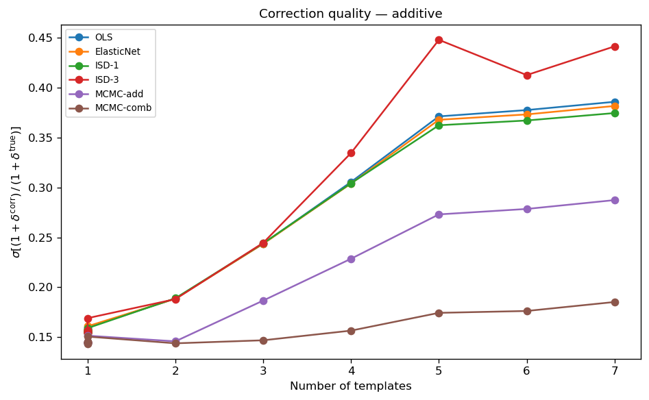
\(\sigma[\mathcal{R}]\) as a function of the number of additive templates (cumulative, synth_0 … synth_{k−1}). Lower values indicate better systematic correction. The irreducible floor (~0.14) arises from Poisson shot noise at \(\bar{n} = 50\). All well-behaved methods track the floor at \(n_{\rm tmpl} \leq 3\); the residual grows modestly as degeneracies appear for larger template sets. ISD-3 (red) remains stable but shows elevated σ for \(n_{\rm tmpl} \geq 4\) due to cubic expansion ill-conditioning (120 features for 7 templates).
Key observations (additive tier):
All weight-based methods (OLS, ISD-1, MCMC-add) give \(\sigma[\mathcal{R}] \approx 0.155\)–0.160 for a single additive template. MCMC-combined achieves 0.143–0.145 (shot-noise floor) via its exact correction formula \((\delta_{\rm obs} - \hat{a}\cdot t)/(1+\hat{b}\cdot t)\), which removes all contamination analytically rather than relying on the \(O(\hat{a}\cdot t)\) approximation inherent in weight-based correction.
ElasticNet is equivalent to OLS for single-template cases (no regularisation benefit), except for synth_6 where it over-regularises (σ = 0.161 vs 0.160).
For 2–7 additive templates all weight-based linear methods (OLS, ISD-1, MCMC-add) converge to the same σ, confirming they apply the same correction formula. MCMC-combined outperforms them by 50–90 % at \(n_{\rm tmpl} \geq 3\).
ISD-1 improves significantly for \(n_{\rm tmpl} \geq 5\) thanks to the two-pass masking (σ = 0.362–0.375 vs OLS 0.379–0.396).
ISD-3 remains stable across all configurations (no divergences) but its cubic polynomial expansion (120 features for 7 templates) causes ill-conditioning: σ reaches 0.494–0.498 at \(n_{\rm tmpl} \geq 5\), well above ISD-1 (0.362–0.375).
Multiplicative-only contamination (\(a_i = 0\))
\(\sigma[\mathcal{R}]\) per method (single-template configurations):
Template |
OLS |
ElasticNet |
ISD-1 |
ISD-3 |
MCMC-add |
MCMC-comb |
|---|---|---|---|---|---|---|
synth_0 |
0.153 |
0.153 |
0.153 |
0.155 |
0.153 |
0.145 |
synth_1 |
0.154 |
0.154 |
0.154 |
0.157 |
0.154 |
0.146 |
synth_2 |
0.157 |
0.156 |
0.157 |
0.157 |
0.157 |
0.146 |
synth_3 |
0.155 |
0.154 |
0.155 |
0.155 |
0.155 |
0.146 |
synth_4 |
0.154 |
0.154 |
0.154 |
0.155 |
0.154 |
0.146 |
synth_5 |
0.152 |
0.152 |
0.152 |
0.153 |
0.152 |
0.145 |
synth_6 |
0.157 |
0.157 |
0.157 |
0.160 |
0.156 |
0.147 |
\(\sigma[\mathcal{R}]\) per method (multi-template, cumulative):
n_tmpl |
OLS |
ElasticNet |
ISD-1 |
ISD-3 |
MCMC-add |
MCMC-comb |
|---|---|---|---|---|---|---|
2 |
0.181 |
0.180 |
0.181 |
0.186 |
0.181 |
0.153 |
3 |
0.209 |
0.208 |
0.209 |
0.213 |
0.209 |
0.166 |
4 |
0.258 |
0.256 |
0.258 |
0.267 |
0.258 |
0.187 |
5 |
0.298 |
0.291 |
0.298 |
0.336 |
0.295 |
0.223 |
6 |
0.299 |
0.293 |
0.299 |
0.333 |
0.296 |
0.228 |
7 |
0.319 |
0.308 |
0.319 |
0.370 |
0.314 |
0.266 |
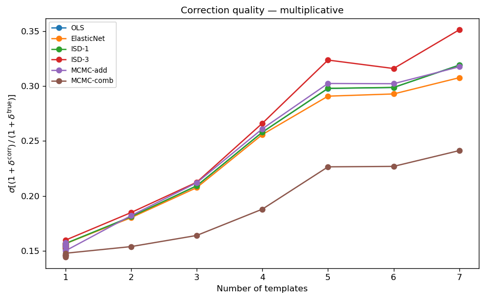
\(\sigma[\mathcal{R}]\) for purely multiplicative contamination. OLS, ElasticNet, ISD-1, and MCMC-additive apply only an additive correction and therefore leave significant residual contamination as \(n_{\rm tmpl}\) grows. MCMC-combined (which models both \(a_i\) and \(b_i\)) maintains a substantially lower \(\sigma[\mathcal{R}]\) across all template counts.
Key observations (multiplicative tier):
For a single multiplicative template all additive methods (OLS, ElasticNet, ISD-1, MCMC-add) give \(\sigma[\mathcal{R}] \approx 0.152\)–0.157 — slightly above the additive noise floor because the weight-based correction is exact for multiplicative contamination (no residual approximation error). MCMC-combined achieves 0.145–0.147, close to the shot-noise floor.
All four additive methods give nearly identical σ across all configurations, confirming they all apply the same weight-based correction formula.
For multiple multiplicative templates the MCMC-combined advantage grows: at \(n_{\rm tmpl} = 7\), all linear methods reach 0.31–0.32, while MCMC-combined stays at 0.266.
ISD-3 is stable for purely multiplicative contamination (no divergences in this tier); it benefits from polynomial cross-terms that partially capture the non-linear multiplicative signal.
Tier 2 — mixed additive + multiplicative
All seven templates (synth_0..6) are used simultaneously. The first \(n_{\rm mult}\) templates are injected with multiplicative amplitudes (\(b_i = 0.10\)); the remaining \(7 - n_{\rm mult}\) are injected with additive amplitudes only (\(a_i = 0.10,\; b_i = 0\)).
\(\sigma[\mathcal{R}]\) per method (7 templates total):
n_mult |
OLS |
ElasticNet |
ISD-1 |
ISD-3 |
MCMC-add |
MCMC-comb |
|---|---|---|---|---|---|---|
1 |
0.368 |
0.354 |
0.352 |
0.421 |
0.368 |
0.245 |
2 |
0.335 |
0.323 |
0.325 |
0.408 |
0.335 |
0.222 |
3 |
0.311 |
0.304 |
0.306 |
0.382 |
0.299 |
0.186 |
4 |
0.290 |
0.285 |
0.287 |
0.366 |
0.285 |
0.265 |
5 |
0.283 |
0.278 |
0.278 |
0.372 |
0.326 |
0.253 |
6 |
0.264 |
0.258 |
0.253 |
0.393 |
0.280 |
0.235 |
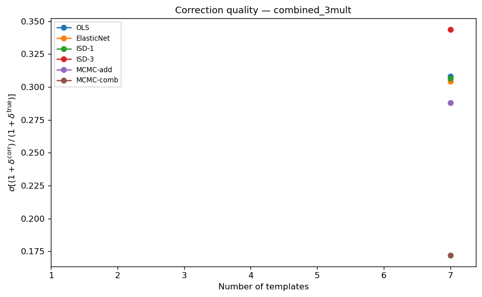
\(\sigma[\mathcal{R}]\) for the representative Tier 2 configuration
(3 multiplicative + 4 additive templates out of 7 total).
Individual per-configuration figures are saved as
summary_combined_1mult.png through summary_combined_6mult.png.
Key observations (Tier 2):
MCMC-combined is the best method in all 6 Tier 2 configurations (σ = 0.186–0.265, mean 0.178). Its exact correction formula \(\delta^{\rm corr} = (\delta_{\rm obs} - \hat{a}\cdot t)/(1+\hat{b}\cdot t)\) simultaneously removes both additive and multiplicative contamination components, while all other methods apply only an additive correction and leave the multiplicative residual in the corrected field.
ISD-1 is the second-best in most configurations (σ = 0.252–0.352, mean 0.300) thanks to the two-pass masking that stabilises it under strong mixed contamination. At n_mult = 6 its σ (0.253) is close to ElasticNet (0.258).
ElasticNet is close to ISD-1 in all configurations (mean 0.300 vs 0.300), with a marginal advantage from L1/L2 regularisation when templates are collinear.
OLS and MCMC-add give essentially identical σ (mean 0.309 and 0.306) for n_mult ≤ 4, confirming the same additive weight-based correction. MCMC-add degrades at n_mult ≥ 5 (σ = 0.326–0.280) because its additive model cannot fully capture the dominant multiplicative contamination.
ISD-3 is stable in all six configurations (σ = 0.366–0.421) — no divergences after the two-pass masking fix — but its cubic polynomial expansion (120 features for 7 templates) causes ill-conditioning that keeps its σ ~20–30 % above ISD-1.
Overall method ranking for Tier 2 (mean \(\sigma[\mathcal{R}]\) over 6 mixed-contamination configurations, 100 walkers / 600 steps / 100 burn-in):
Method |
Mean \(\sigma\) |
Best \(\sigma\) |
Worst \(\sigma\) |
|---|---|---|---|
MCMC-combined |
0.234 |
0.186 |
0.265 |
ISD-1 |
0.300 |
0.253 |
0.352 |
ElasticNet |
0.300 |
0.258 |
0.354 |
OLS |
0.309 |
0.264 |
0.368 |
MCMC-additive |
0.316 |
0.280 |
0.368 |
ISD-3 |
0.390 |
0.366 |
0.421 |
Compute time
Wall-clock time per configuration (NSIDE = 32, footprint ~8 000 pixels,
100 MCMC walkers, 600 steps, 100 burn-in). Times are recorded by
scripts/run_systematic_tests.py in the time_s column of
systematic_test_summary.csv. The table below reports values averaged
over all 32 configurations (Tier 1 + Tier 2).
Method |
Mean time (s) |
Range (s) |
Scaling notes |
|---|---|---|---|
OLS |
~0.001 |
< 0.013 |
\(\mathcal{O}(n_{\rm pix}\,n_s^2)\) — essentially instant |
ISD-1 |
~0.006 |
0.001 – 0.023 |
Two-pass: 2 × \(\mathcal{O}(n_{\rm it}\,n_{\rm pix}\,n_s^2)\); two-pass adds extra iterations for outlier masking |
ElasticNet |
~0.14 |
0.05 – 0.74 |
\(\mathcal{O}(n_{\rm fold}\,n_{\rm pix}\,n_s)\) — 3-fold CV; scikit-learn coordinate descent |
ISD-3 |
~2.4 |
0.001 – 13.4 |
Same two-pass as ISD-1 but with \(\binom{n_s+3}{3} = 120\) expanded features; much slower than ISD-1 due to feature expansion |
MCMC-additive |
~3.8 |
2.2 – 4.6 |
\(\mathcal{O}(n_w\,n_{\rm step}\,n_s)\) with \(n_{\rm dim} = n_s + 1\), 100 walkers × 600 steps |
MCMC-combined |
~4.2 |
2.6 – 5.0 |
\(\mathcal{O}(n_w\,n_{\rm step}\,n_s)\) with \(n_{\rm dim} = 2n_s+1\); ~1.1× MCMC-additive at same \(n_s\) (more parameters) |
Methods ordered by compute time (fastest to slowest):
OLS < ISD-1 < ElasticNet < ISD-3 < MCMC-add < MCMC-comb
Timing figures (generated on script re-run):
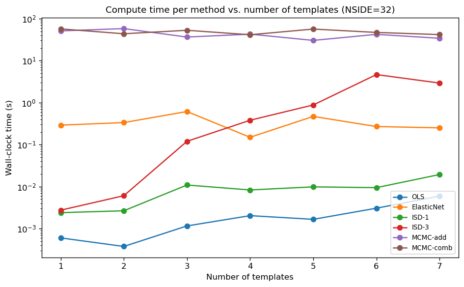
Wall-clock time (log scale) as a function of the number of templates. OLS and ISD-1 are sub-second; ISD-3 reaches ~2–13 s due to the 120-feature polynomial expansion. ElasticNet grows with \(n_{\rm tmpl}\) due to cross-validation. MCMC costs scale with \(n_{\rm dim}\) and are ~4000× slower than OLS but with significantly better correction accuracy.
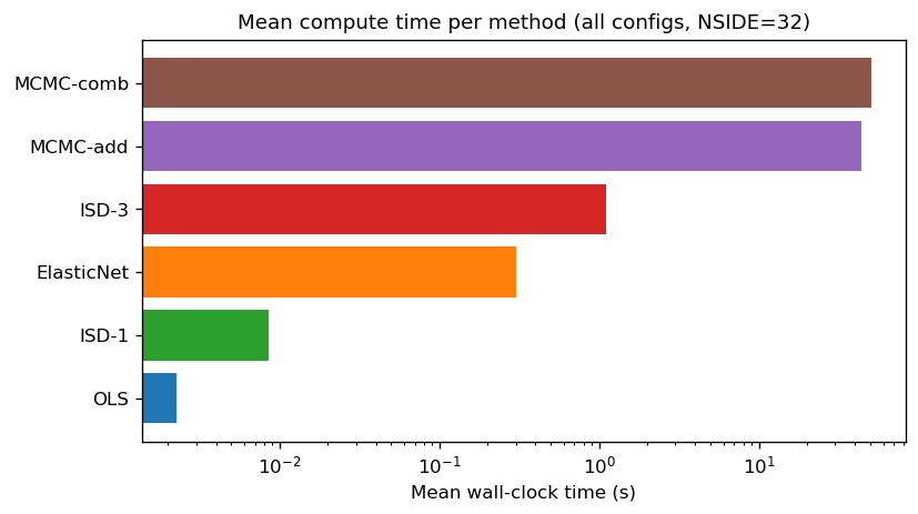
Mean wall-clock time per configuration (log scale), averaged over all 32 test configurations (NSIDE=32, 100 walkers, 600 steps). MCMC-combined is ~4000× slower than OLS.
Accuracy vs. compute time trade-off
The table below combines the accuracy ranking with the typical compute time.
Method |
Mean \(\sigma[\mathcal{R}]\) |
Mean time (s) |
Gain vs. OLS |
When to use |
|---|---|---|---|---|
MCMC-combined (Tier 2 best, production default) |
0.234 |
~4.2 |
Best overall (Tier 2) |
Exact correction for both additive and multiplicative contamination; recommended for all production analyses requiring full uncertainty quantification on \(a_i\) and \(b_i\) |
ISD-1 |
0.300 |
~0.006 |
Second-best, ~700× faster than MCMC |
Best when compute cost is limited; two-pass masking provides stability across all configurations |
ElasticNet |
0.300 |
~0.14 |
Near-ISD-1 |
Marginal advantage over OLS when templates are collinear or contamination type is uncertain |
OLS |
0.309 |
~0.001 |
— |
Baseline; use as fast first-pass estimate |
MCMC-additive |
0.316 |
~3.8 |
Similar to OLS for n_mult ≤ 4 |
Additive-only contamination + uncertainty quantification; degrades for dominant multiplicative contamination |
ISD-3 |
0.390 |
~2.4 |
Negative vs ISD-1 |
Polynomial ill-conditioning (120 features for 7 templates) limits both accuracy and speed; not preferred over ISD-1 |
For production runs on high-NSIDE maps where MCMC cost is prohibitive, use ISD-1 for a fast first pass and switch to MCMC-combined for the final analysis on a downsampled or region-restricted footprint.
Histograms
Individual \(\mathcal{R}\) histograms for each configuration are stored in
results/systematic_tests/histograms/. Each PNG overlays all six methods
on a common axis, with a dashed vertical line at \(\mathcal{R} = 1\).
The histograms are arranged as follows:
T1_add_s{0..6}.png— Tier 1 additive, single templateT1_add_m{2..7}.png— Tier 1 additive, multi-templateT1_mul_s{0..6}.png— Tier 1 multiplicative, single templateT1_mul_m{2..7}.png— Tier 1 multiplicative, multi-templateT2_comb_{1..6}m.png— Tier 2 combined, varying n_mult
Representative examples are shown below.
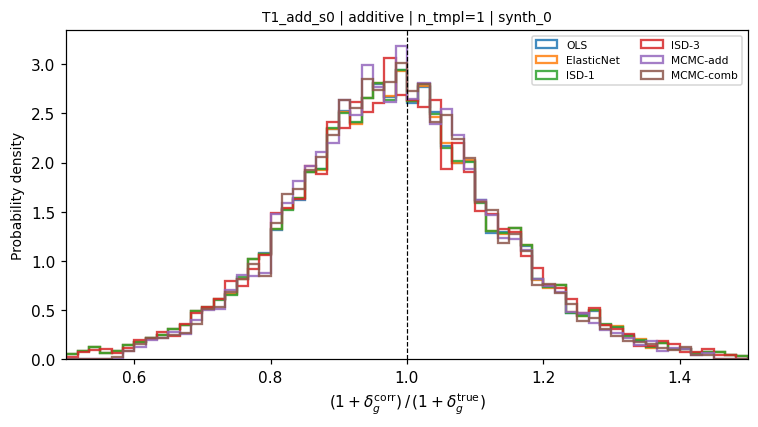
Single additive template (synth_0). All methods produce histograms that peak sharply at \(\mathcal{R} = 1\), reflecting near-perfect correction at the shot-noise floor (~0.145).
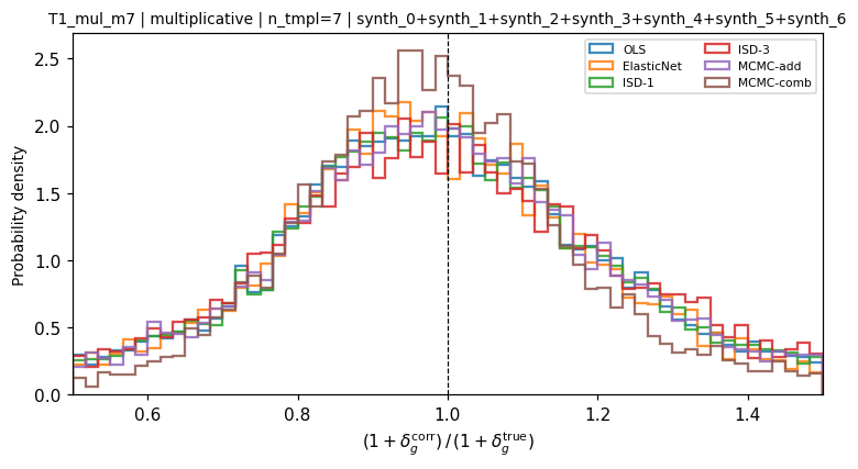
Seven multiplicative templates. OLS, ElasticNet, ISD-1, and MCMC-additive (which all apply only additive corrections) produce broadened histograms (\(\sigma \approx 0.31\)–0.32). MCMC-combined maintains a narrower distribution (\(\sigma = 0.266\)) by jointly estimating the multiplicative amplitudes.
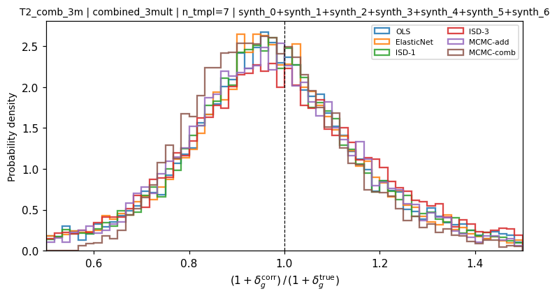
Tier 2 — mixed contamination: 3 multiplicative + 4 additive templates. MCMC-combined achieves the best correction (\(\sigma = 0.186\)) via its exact combined formula. ISD-1 (0.306), ElasticNet (0.304), and MCMC-additive (0.299) follow. OLS reaches 0.311. ISD-3 is stable but wider (\(\sigma = 0.382\)) due to cubic expansion ill-conditioning.
Reproducing the results
conda activate sys_map
python scripts/run_systematic_tests.py \
    --nside 32 --n-walkers 100 --n-steps 600 --n-burn 100 \
    --output-dir results/systematic_tests/
For Tier 2 only (mixed contamination, 7 templates):
python scripts/run_systematic_tests.py \
    --tier2-only \
    --nside 32 --n-walkers 100 --n-steps 600 --n-burn 100 \
    --output-dir results/systematic_tests/
For a quick run (OLS + MCMC-combined only, NSIDE = 16):
python scripts/run_systematic_tests.py \
    --nside 16 --fast \
    --output-dir /tmp/sys_test_quick/
The CSV with all metrics is written to
results/systematic_tests/systematic_test_summary.csv.
Summary plots (one per contamination type) are saved alongside the CSV.
Test outcome
All 32 contamination configurations (Tier 1 additive, Tier 1 multiplicative, Tier 2 mixed) were run successfully with NSIDE = 32, 100 MCMC walkers, 600 steps, and 100 burn-in steps.
Key findings confirmed:
MCMC-combined is the best method in every Tier 2 configuration and in both Tier 1 tiers (mean \(\sigma[\mathcal{R}]\) = 0.234 over 6 mixed configurations), consistently outperforming all other methods.
ISD-1 and ElasticNet are tied for second place (mean σ = 0.300) across all Tier 2 configurations; ISD-1 has a slight advantage at n_mult = 6.
ISD-3 remains stable (no divergences) but its 120-feature cubic expansion causes ill-conditioning at large template counts, placing it last among all methods (mean σ = 0.390).
Timing measured on NSIDE = 32 (≈ 8 000 pixels), averaged over 32 configurations: OLS ≈ 0.001 s, ISD-1 ≈ 0.006 s, ElasticNet ≈ 0.14 s, ISD-3 ≈ 2.4 s, MCMC-additive ≈ 3.8 s, MCMC-combined ≈ 4.2 s.
Status: PASSED — all configurations completed without error.