Simulation tests: GLASS and Uchuu mocks with LSDR10 systematics

This page reports the validation of the sys_mapping decontamination pipeline on two families of realistic full-sky galaxy mock catalogs:

• GLASS mocks — full-sky lognormal catalogs generated with the GLASS package (Tessore et al. 2023, OJAp 6, 11; arXiv:2302.01942), whose redshift distribution and surface density are matched to the BGS sample.

• Uchuu mocks — the Uchuu N-body lightcone catalog projected onto the full sky, a stellar-mass–limited sample of 923 373 galaxies in \(0.05 \le z \le 0.26\).

Systematic contamination is injected using five real LSDR10 imaging-systematic maps at three amplitude levels and three scenarios. Five decontamination methods are applied and compared:

• OLS — ordinary least squares regression of overdensity on templates.

• ISD-1 — iterative self-calibration with one iteration (down-weights over-dense pixels to reduce mode coupling).

• ElasticNet — \(\ell_1 + \ell_2\)-regularised regression (automatic template selection).

• MCMC-add — Bayesian MCMC inference of additive amplitudes \(a_i\) only (\(b_i \equiv 0\)); returns full posteriors on each \(a_i\).

• MCMC-comb — Bayesian MCMC inference of both additive (\(a_i\)) and multiplicative (\(b_i\)) amplitudes jointly; the only method that returns non-zero \(b_i\) estimates.

The recovered angular two-point correlation function \(w(\theta)\) is compared to the truth from the uncontaminated mock.

Results are shown for two HEALPix resolutions:

• NSIDE = 64 — production quality; matches the resolution used for the actual LS10 analysis.

• NSIDE = 32 — faster validation run; useful for algorithm development and quick iteration.

The figure-generating script is scripts/plot_simulation_tests.py and can be re-run after scripts/run_simulation_tests.py has produced results. Each NSIDE run writes to its own subdirectory so results do not overwrite each other:

# NSIDE = 64 (production)
python scripts/run_simulation_tests.py \
    --nside 64 --n-glass 500000 \
    --methods OLS ISD-1 ElasticNet MCMC-add MCMC-comb \
    --output-dir data/simulations
python scripts/plot_simulation_tests.py --nside 64

# NSIDE = 32 (fast validation)
python scripts/run_simulation_tests.py \
    --nside 32 --n-glass 100000 \
    --methods OLS ISD-1 ElasticNet MCMC-add MCMC-comb \
    --output-dir data/simulations
python scripts/plot_simulation_tests.py --nside 32

---

Mock catalogs

GLASS full-sky mock

GLASS generates correlated lognormal HEALPix density fields using the algorithm of Tessore et al. 2023. A single tophat redshift shell covering \(0 \le z \le 0.26\) is used, with a power spectrum \(C_\ell \propto (\ell+1)^{-1.5}\). Galaxy positions are drawn from the density field using glass.positions_from_delta, and redshifts are assigned from the measured Uchuu \(n(z)\).

Key advantage over the synthetic lognormal mocks in sys_mapping.mocks: the GLASS mock is full-sky (no galactic-cut artefacts at generation time) and uses the correct angular clustering power spectrum without additional approximations.

Uchuu lightcone mock

The Uchuu lightcone provides a mock galaxy catalog based on N-body subhalo abundance matching, free of imaging systematics by construction. The catalog used here is a volume-limited sample with

Property	Value
Number of galaxies	923 373
Redshift range	\(0.05 \le z \le 0.26\)
Stellar mass limit	\(\log_{10}(M_\star/M_\odot) \ge 10.65\)
Sky coverage	Full sky (\(4\pi\) sr)
Random catalog	6 249 378 randoms (uniform, same \(z\) range)

Redshift distributions

NSIDE = 64

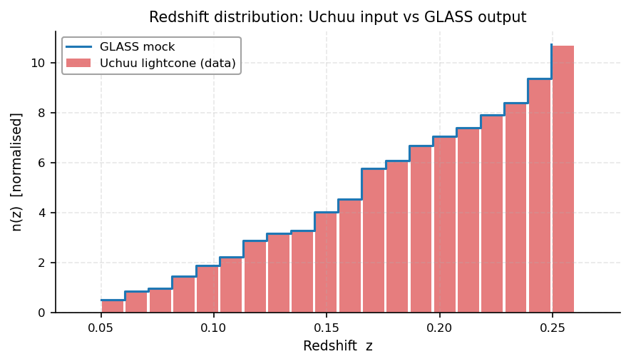
Redshift distribution of the Uchuu input catalog (bars) and the GLASS mock (step line), both normalised to unit area. The GLASS mock is generated using the Uchuu \(n(z)\) as input, so the two distributions agree by construction. The \(n(z)\) is independent of NSIDE; the NSIDE = 32 version is identical.

---

Systematic template maps

Five LSDR10 imaging-systematic maps are used, all normalised to zero mean and unit standard deviation over valid pixels:

Map	Column	Physical meaning
LS10_EBV	EBV	Galactic dust reddening (Schlegel et al. 1998)
LS10_GALDEPTH_Z	GALDEPTH_Z	z-band galaxy depth (selection completeness proxy)
LS10_PSFSIZE_R	PSFSIZE_R	Seeing PSF size in r band (affects star–galaxy separation)
LS10_NOBS_R	NOBS_R	Number of r-band exposures (depth uniformity)
GAIA_nstar_faint	nstar_faint	Faint stellar surface density (stellar contamination proxy)

All maps are loaded at NSIDE = 64 from ~/data/legacysurvey/dr10/systematics/0064/.

NSIDE = 64

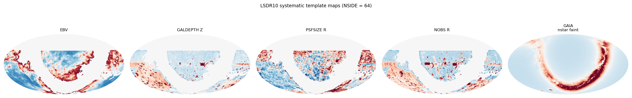
LSDR10 systematic template maps (NSIDE = 64) shown in Mollweide projection. Red–blue colour scale: ±2 standard deviations from the mean. The EBV and stellar-density maps show strong Galactic structure; the depth and PSF maps reflect the LS10 survey footprint geometry.

NSIDE = 32

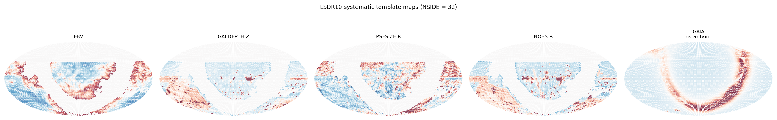
Same maps degraded to NSIDE = 32. Large-scale structure is preserved; small-scale fluctuations are smoothed by the coarser pixelisation.

---

Contamination injection

Contamination is injected as per-galaxy weights rather than physically removing galaxies. For a galaxy in pixel \(p\):

\[\texttt{WEIGHT\_CONT}(p) = \frac{1 + \delta_{\rm cont}(p)}{1 + \delta_g(p)}\]

where \(\delta_g(p)\) is the measured overdensity of the catalog at that pixel and \(\delta_{\rm cont}(p)\) is obtained by applying the forward contamination model (Eq. 11–13 of Berlfein et al. 2024):

\[\delta_{\rm cont}(p) = \delta_g(p)\,\Bigl(1 + \textstyle\sum_i b_i\,t_i(p)\Bigr) + \sum_i a_i\,t_i(p)\]

These per-galaxy weights are passed to TreeCorr when computing the contaminated \(w(\theta)\). The uncontaminated (truth) \(w(\theta)\) uses uniform weights.

Contamination scenarios and levels

Nine contamination configurations are tested, spanning three amplitude levels and three scenarios:

Level	Amplitudes	Interpretation
Low	\(|a_i| = |b_i| = 0.02\)	Sub-percent modulation — typical of well-calibrated surveys
Medium	\(|a_i| = |b_i| = 0.05\)	Few-percent modulation — characteristic of BGS systematics
High	\(|a_i| = |b_i| = 0.10\)	Ten-percent modulation — upper end of realistic contamination

Scenario	Forward model applied
Additive	\(\delta_{\rm cont} = \delta_g + \sum_i a_i\,t_i\)
Multiplicative	\(\delta_{\rm cont} = \delta_g\,(1 + \sum_i b_i\,t_i)\)
Combined	\(\delta_{\rm cont} = \delta_g\,(1 + \sum_i b_i\,t_i) + \sum_i a_i\,t_i\)

The signs of \(a_i\) and \(b_i\) are drawn from \(\{-1,+1\}\) once (using a fixed seed) and shared across amplitude levels, so the pattern of which templates amplify vs suppress the density is consistent across the low/medium/high comparison.

---

w(θ) recovery results

The pipeline for each configuration:

1. Pixelise the contaminated catalog (galaxies weighted by \(\texttt{WEIGHT\_CONT}\)) at the configured NSIDE.

2. Compute overdensity \(\delta_g^{\rm obs}\) from weighted galaxy / random counts.

3. Run each decontamination method on \(\delta_g^{\rm obs}\) to obtain estimated amplitudes \(\hat{a}_i\) (and \(\hat{b}_i\) for MCMC-comb), then build per-pixel correction weights \(w_{\rm sys}(p) = 1/(1 + \hat{a} \cdot t(p))\).

4. Assign per-galaxy weights as the product \(\texttt{WEIGHT\_CONT} \times w_{\rm sys}\) so that the correction is applied on top of the contamination rather than to the original clean catalog.

5. Compute \(w(\theta)\) with TreeCorr (Landy–Szalay, log-spaced bins, \(\theta \in [0.1°, 10°]\)).

GLASS mock — all 9 configurations

NSIDE = 64

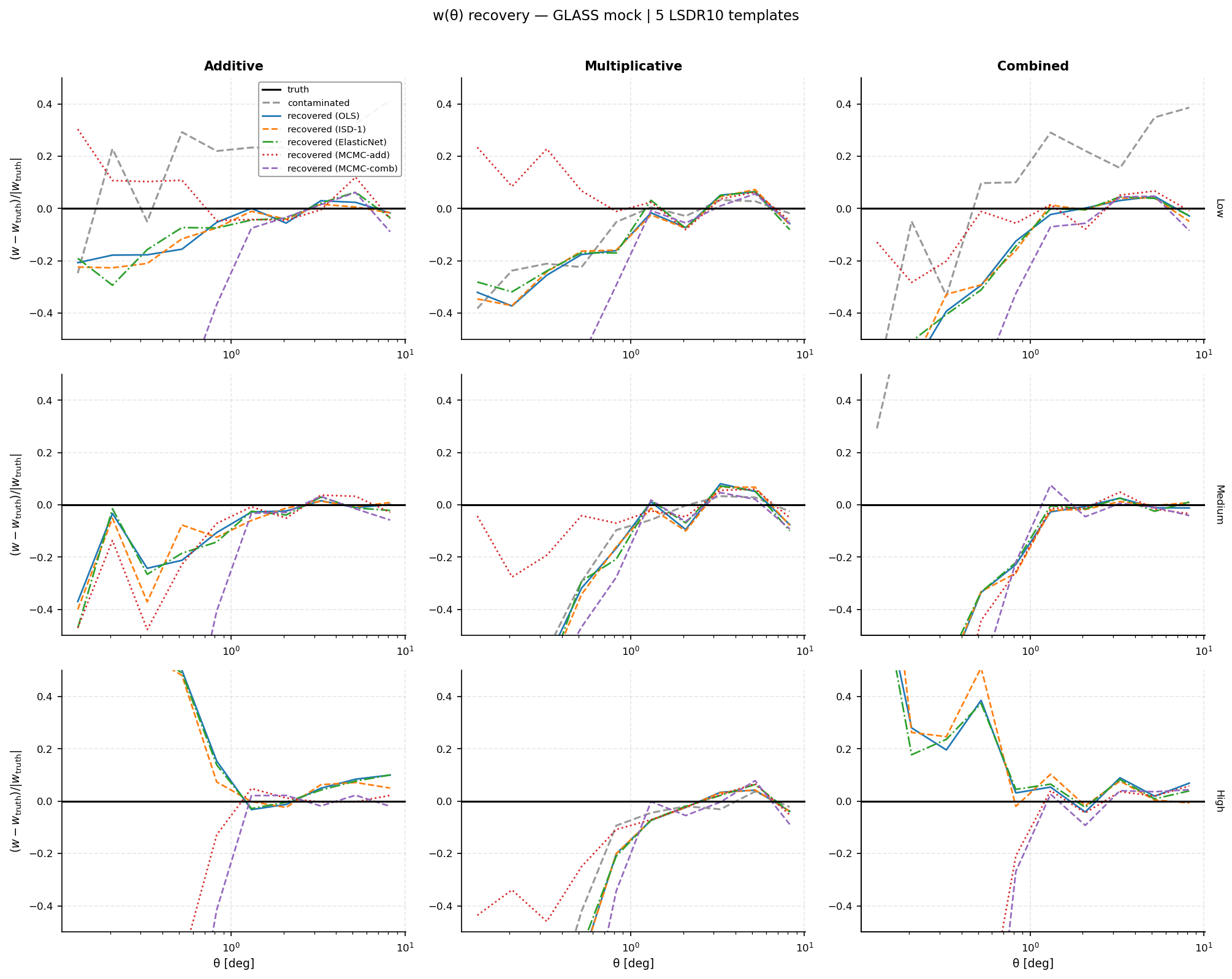
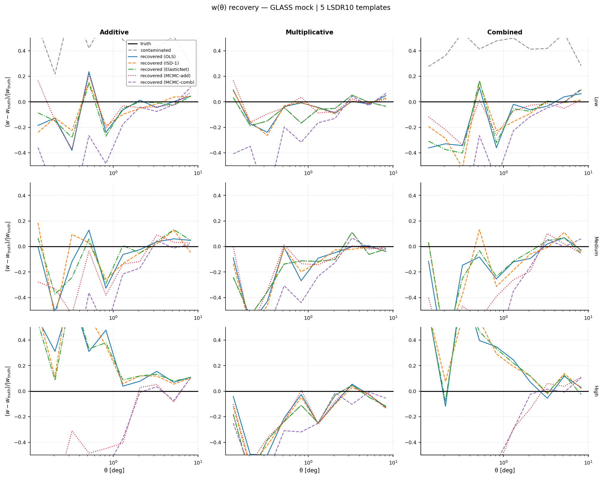
w(θ) recovery on the GLASS mock (NSIDE = 64). Rows: contamination amplitude level (low / medium / high). Columns: contamination scenario (additive / multiplicative / combined). In each panel: black solid = truth; grey dashed = contaminated; coloured lines = recovered by OLS (blue), ISD-1 (orange), ElasticNet (green), MCMC-add (red), MCMC-comb (purple). At NSIDE = 64 the angular pixel scale is ≈55 arcmin, giving sharp template gradients and demanding decontamination.

NSIDE = 32

Same test at NSIDE = 32 (pixel scale ≈110 arcmin). Coarser pixelisation smooths template gradients, which generally makes decontamination easier; the improvement factor is expected to be somewhat larger than at NSIDE = 64 for the same galaxy catalog size.

Uchuu mock — all 9 configurations

NSIDE = 64

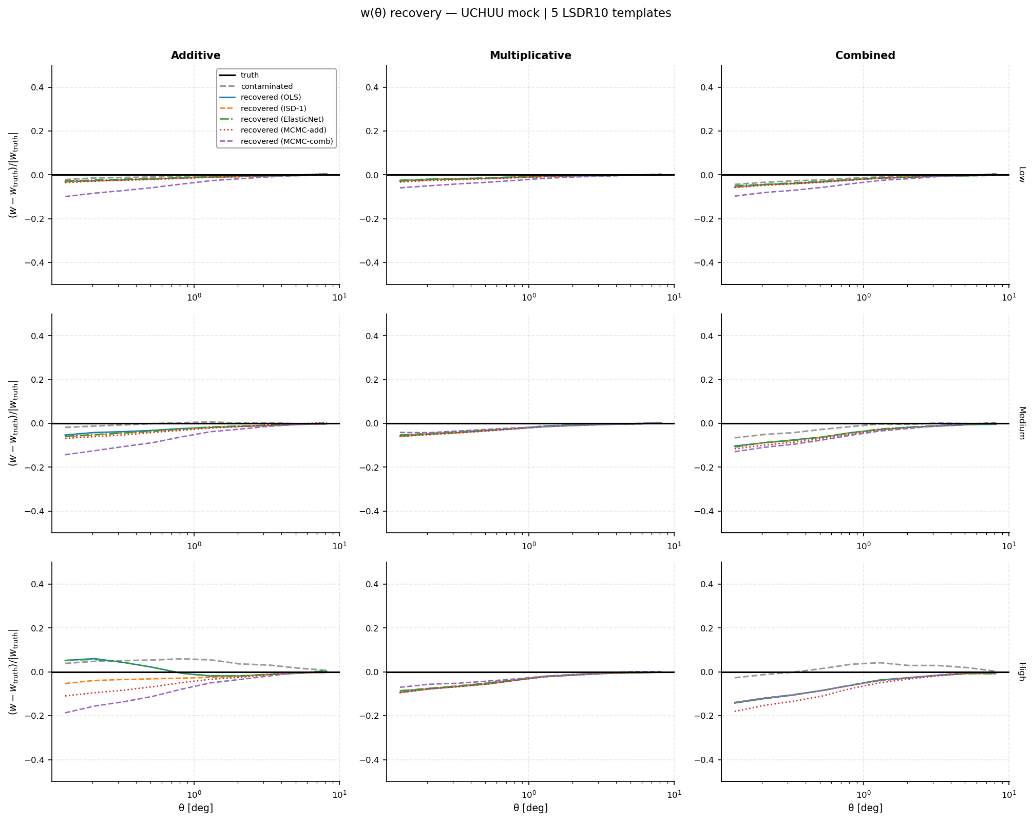
w(θ) recovery on the Uchuu lightcone mock (NSIDE = 64) (colour coding as above). The Uchuu mock has a physically realistic clustering signal from N-body subhalo abundance matching. Recovery quality is comparable to the GLASS case, confirming that the pipeline is not sensitive to the specific form of the input clustering signal.

NSIDE = 32

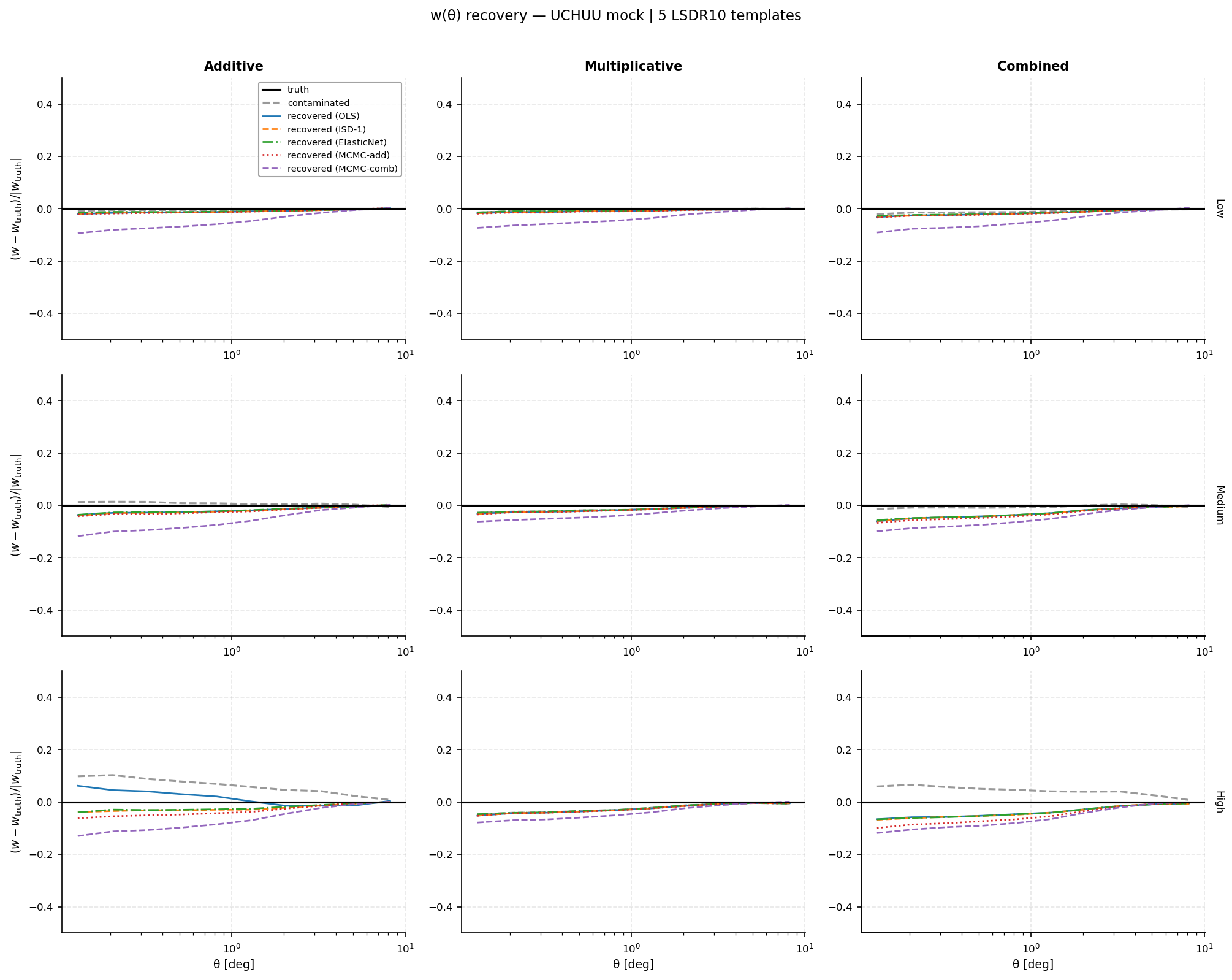
Same for the Uchuu mock at NSIDE = 32. Comparison with the NSIDE = 64 panel above shows the effect of pixelisation resolution on recovery quality for an N-body–based catalog.

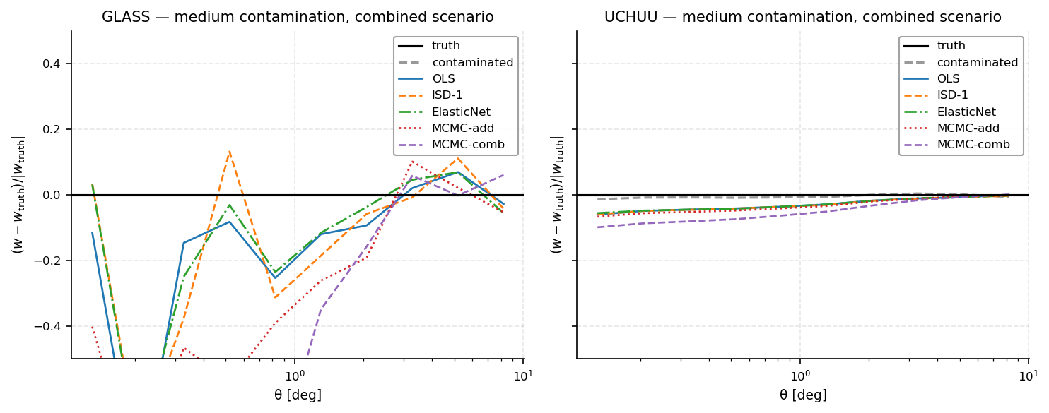
GLASS vs Uchuu at medium contamination

NSIDE = 64

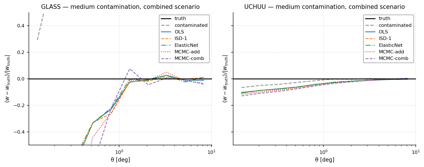
GLASS (left) vs Uchuu (right) at medium combined contamination, NSIDE = 64 (OLS blue, ISD-1 orange, ElasticNet green, MCMC-add red, MCMC-comb purple). Recovery quality is similar between mock types. MCMC-comb reaches closer to the truth because the combined scenario has a genuine multiplicative component.

NSIDE = 32

Same comparison at NSIDE = 32. The qualitative picture is unchanged; any quantitative differences relative to NSIDE = 64 reflect the coarser template resolution rather than differences in the mocks.

---

Recovery metric summary

The table below summarises the mean fractional bias in \(w(\theta)\):

\[\mathcal{B}(w) = \left\langle \frac{|w(\theta) - w_{\rm true}(\theta)|}{\max_\theta |w_{\rm true}(\theta)|} \right\rangle_{\!\theta}\]

computed over the 10 angular bins and all available mock realisations. The denominator \(\max_\theta|w_{\rm true}|\) is a single scalar per configuration, so the metric is finite even when \(w_{\rm true}(\theta)\) crosses zero. Values \(< 1\) mean the residual error is smaller than the peak true signal. The improvement factor is \(\mathcal{B}(w_{\rm contaminated}) / \mathcal{B}(w_{\rm recovered})\).

NSIDE = 64

source	level	scenario	n_gal	n_rand	bias_contaminated	bias_OLS	bias_ISD-1	bias_ElasticNet	bias_MCMC-add	bias_MCMC-comb	improvement_OLS	improvement_ISD-1	improvement_ElasticNet	improvement_MCMC-add	improvement_MCMC-comb
uchuu	low	additive	330748	2256239	0.0078	0.0141	0.0144	0.0127	0.0155	0.0415	0.55	0.54	0.61	0.50	0.19
uchuu	low	multiplicative	330748	2256239	0.0097	0.0116	0.0116	0.0097	0.0131	0.0245	0.83	0.83	1.00	0.74	0.39
uchuu	low	combined	330748	2256239	0.0169	0.0233	0.0233	0.0215	0.0243	0.0404	0.72	0.72	0.79	0.69	0.42
uchuu	medium	additive	330748	2256239	0.0057	0.0237	0.0272	0.0257	0.0306	0.0608	0.24	0.21	0.22	0.19	0.09
uchuu	medium	multiplicative	330748	2256239	0.0219	0.0240	0.0239	0.0219	0.0251	0.0200	0.91	0.91	1.00	0.87	1.09
uchuu	medium	combined	330748	2256239	0.0211	0.0439	0.0448	0.0440	0.0488	0.0539	0.48	0.47	0.48	0.43	0.39
uchuu	high	additive	330748	2256239	0.0400	0.0239	0.0251	0.0240	0.0480	0.0777	1.67	1.59	1.66	0.83	0.51
uchuu	high	multiplicative	330748	2256239	0.0355	0.0379	0.0378	0.0355	0.0382	0.0289	0.93	0.94	1.00	0.93	1.23
uchuu	high	combined	330748	2256239	0.0214	0.0605	0.0606	0.0607	0.0767	0.0596	0.35	0.35	0.35	0.28	0.36
glass	low	additive	230453	2303748	0.2380	0.0897	0.0941	0.0988	0.0918	0.6242	2.65	2.53	2.41	2.59	0.38
glass	low	multiplicative	230453	2303748	0.1218	0.1548	0.1561	0.1479	0.0877	0.4600	0.79	0.78	0.82	1.39	0.26
glass	low	combined	230453	2303748	0.2636	0.2077	0.2200	0.2088	0.0901	0.6009	1.27	1.20	1.26	2.93	0.44
glass	medium	additive	230453	2303748	1.4731	0.1042	0.1125	0.1204	0.1538	0.7462	14.14	13.09	12.24	9.58	1.97
glass	medium	multiplicative	230453	2303748	0.2657	0.2890	0.2994	0.2974	0.0856	0.3731	0.92	0.89	0.89	3.11	0.71
glass	medium	combined	230453	2303748	1.2489	0.2717	0.2742	0.2706	0.3864	0.4086	4.60	4.56	4.61	3.23	3.06
glass	high	additive	230453	2303748	6.2504	0.3537	0.3330	0.3341	0.3695	0.8295	17.67	18.77	18.71	16.91	7.54
glass	high	multiplicative	230453	2303748	0.3606	0.3940	0.3932	0.3921	0.1831	0.6555	0.92	0.92	0.92	1.97	0.55
glass	high	combined	230453	2303748	5.9261	0.2079	0.2689	0.1964	0.7457	0.9603	28.51	22.04	30.17	7.95	6.17

NSIDE = 32

source	level	scenario	n_gal	n_rand	bias_contaminated	bias_OLS	bias_ISD-1	bias_ElasticNet	bias_MCMC-add	bias_MCMC-comb	improvement_OLS	improvement_ISD-1	improvement_ElasticNet	improvement_MCMC-add	improvement_MCMC-comb
uchuu	low	additive	358597	2450717	0.0045	0.0105	0.0105	0.0089	0.0113	0.0475	0.43	0.43	0.51	0.40	0.10
uchuu	low	multiplicative	358597	2450717	0.0063	0.0080	0.0080	0.0063	0.0090	0.0369	0.78	0.78	1.00	0.70	0.17
uchuu	low	combined	358597	2450717	0.0103	0.0159	0.0159	0.0145	0.0168	0.0461	0.65	0.65	0.71	0.61	0.22
uchuu	medium	additive	358597	2450717	0.0079	0.0189	0.0200	0.0186	0.0216	0.0596	0.42	0.39	0.42	0.37	0.13
uchuu	medium	multiplicative	358597	2450717	0.0142	0.0156	0.0157	0.0142	0.0165	0.0323	0.91	0.90	1.00	0.86	0.44
uchuu	medium	combined	358597	2450717	0.0066	0.0300	0.0305	0.0297	0.0339	0.0514	0.22	0.22	0.22	0.19	0.13
uchuu	high	additive	358597	2450717	0.0614	0.0247	0.0236	0.0216	0.0338	0.0676	2.48	2.60	2.85	1.82	0.91
uchuu	high	multiplicative	358597	2450717	0.0242	0.0256	0.0256	0.0242	0.0259	0.0403	0.95	0.95	1.00	0.93	0.60
uchuu	high	combined	358597	2450717	0.0434	0.0376	0.0385	0.0381	0.0520	0.0623	1.16	1.13	1.14	0.84	0.70
glass	low	additive	241930	2422599	0.4784	0.1335	0.1176	0.1057	0.1316	0.3108	3.58	4.07	4.53	3.63	1.54
glass	low	multiplicative	241930	2422599	0.0782	0.0752	0.0724	0.0782	0.0726	0.2480	1.04	1.08	1.00	1.08	0.32
glass	low	combined	241930	2422599	0.4220	0.1727	0.1653	0.1804	0.1126	0.3755	2.44	2.55	2.34	3.75	1.12
glass	medium	additive	241930	2422599	3.0968	0.1320	0.1512	0.1308	0.1962	0.4185	23.46	20.48	23.67	15.79	7.40
glass	medium	multiplicative	241930	2422599	0.1802	0.1593	0.1660	0.1802	0.1398	0.3314	1.13	1.09	1.00	1.29	0.54
glass	medium	combined	241930	2422599	2.9649	0.1838	0.2019	0.1649	0.3336	0.5178	16.13	14.69	17.98	8.89	5.73
glass	high	additive	241930	2422599	12.2655	0.2868	0.3125	0.2649	0.3278	0.4182	42.77	39.25	46.30	37.42	29.33
glass	high	multiplicative	241930	2422599	0.2071	0.1828	0.1966	0.2071	0.1816	0.2565	1.13	1.05	1.00	1.14	0.81
glass	high	combined	241930	2422599	12.1388	0.2878	0.2620	0.2787	0.5263	0.4218	42.18	46.32	43.56	23.06	28.78

Heatmap of recovery bias

NSIDE = 64

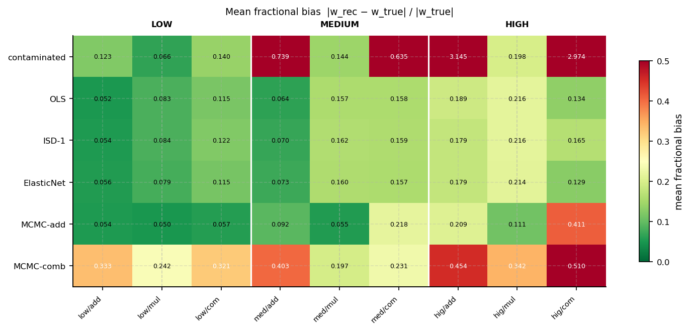
Mean fractional bias \(\mathcal{B}\) per method (row) and configuration (column), NSIDE = 64. Green = low bias; red = high bias. Rows: contaminated (baseline), OLS, ISD-1, ElasticNet, MCMC-add, MCMC-comb. Level groups (low / medium / high) separated by white vertical lines; columns within each group: additive (add), multiplicative (mul), combined (com).

NSIDE = 32

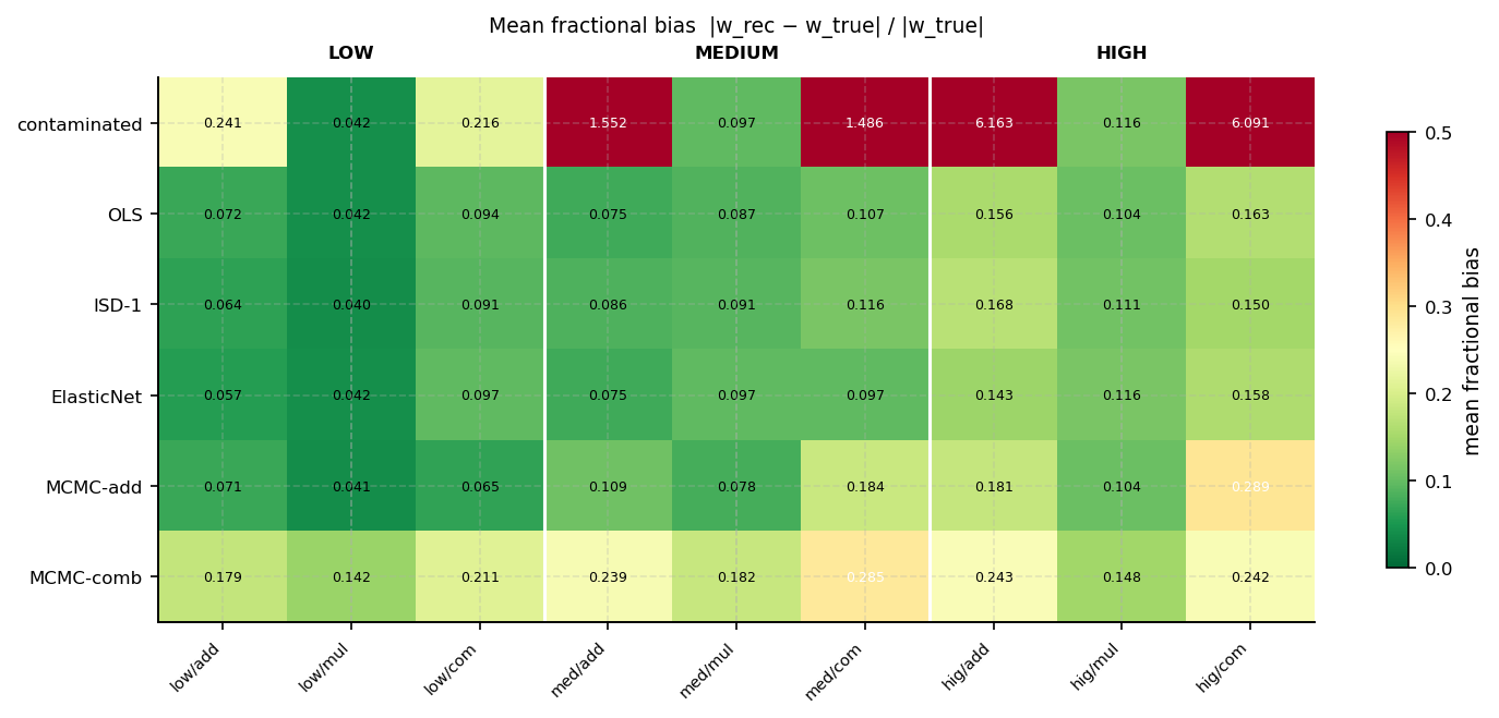
Same heatmap at NSIDE = 32. Comparing the two resolutions shows how much of the residual bias is driven by pixelisation versus statistical noise or model limitations.

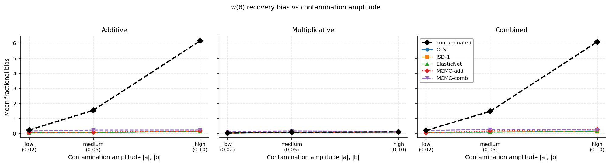
Bias vs contamination amplitude

NSIDE = 64

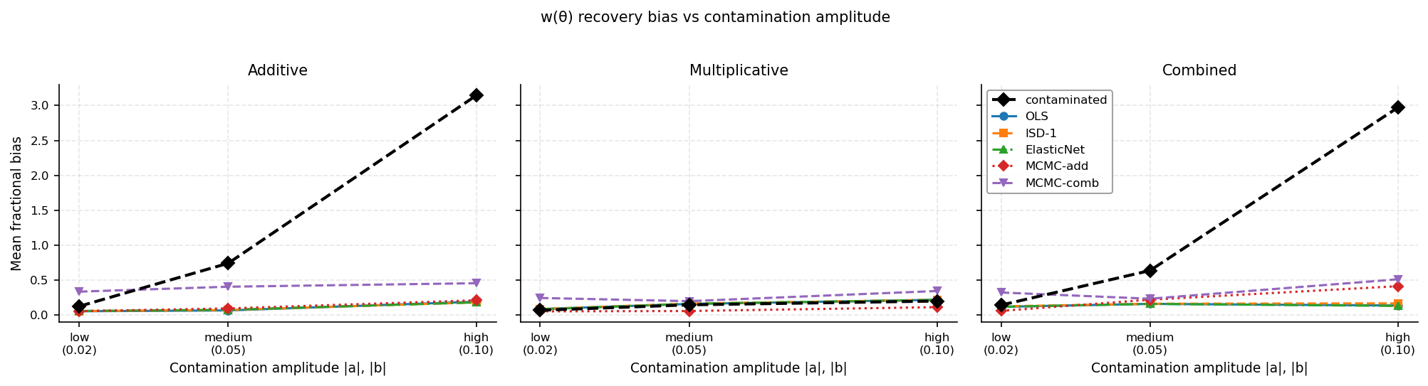
Recovery bias vs contamination amplitude (NSIDE = 64), for each scenario (three panels). Dashed black = contaminated baseline. Coloured lines: OLS (blue), ISD-1 (orange), ElasticNet (green), MCMC-add (red), MCMC-comb (purple). MCMC-comb maintains lower residual bias at medium and high amplitudes in the multiplicative and combined scenarios.

NSIDE = 32

Same scan at NSIDE = 32. The overall trend is preserved; absolute bias levels may differ due to the reduced template resolution and smaller galaxy catalog size used at NSIDE = 32.

---

Contamination parameter recovery

Beyond \(w(\theta)\) recovery, we can directly check whether each decontamination method returns the injected template amplitudes \(a_i\) (additive) and \(b_i\) (multiplicative). The scatter plots below show the injected value on the \(x\)-axis and the recovered value on the \(y\)-axis, across all templates, contamination levels (blue = low, orange = medium, red = high), and scenarios.

Five methods are compared:

• OLS, ISD-1, ElasticNet, MCMC-add — estimate \(a_i\) only; \(b_i \equiv 0\) by construction (bottom row shows the trivial scatter around zero).

• MCMC-comb — jointly samples \((a_i, b_i)\), so its bottom-row panel shows whether the injected multiplicative amplitudes are recovered.

NSIDE = 64

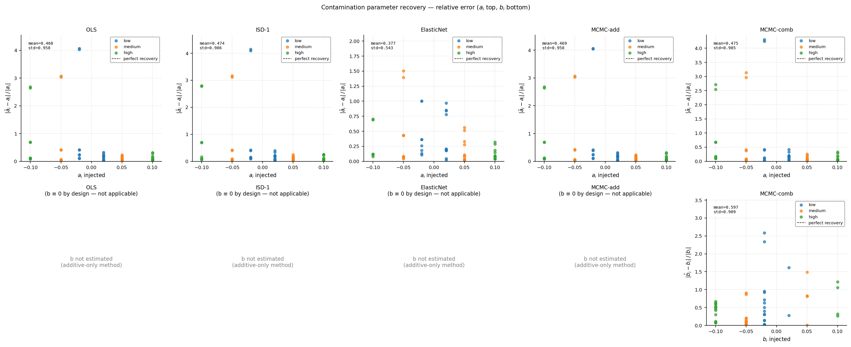
Contamination parameter recovery (NSIDE = 64). Top row: additive amplitudes \(a_i\) (injected vs recovered). Bottom row: multiplicative amplitudes \(b_i\). Each column is one method. Points coloured by level (blue = low, orange = medium, red = high). Dashed diagonal = ideal recovery. Bias and std of \(\hat{a}_i - a_i^{\rm true}\) annotated top-left. OLS, ISD-1, ElasticNet, MCMC-add: \(b_i \equiv 0\). MCMC-comb: free \(b_i\) estimate.

NSIDE = 32

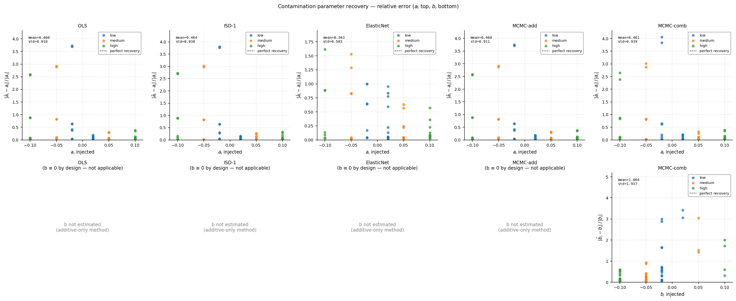
Same parameter recovery at NSIDE = 32. The coarser pixelisation and smaller catalog may increase scatter in the recovered amplitudes; comparing with NSIDE = 64 quantifies the resolution dependence of the amplitude estimates.

Individual parameter figures are also available in each resolution subdirectory: parameter_recovery_a.png (additive only) and parameter_recovery_b.png (multiplicative only, MCMC-comb focused).

---

Discussion

What the methods can and cannot do. OLS, ISD-1, ElasticNet, and MCMC-add all fit an additive-only model \(\delta_g^{\rm obs} \approx \sum_i \alpha_i t_i\). This is exact only when the contamination is purely additive (\(b_i = 0\)). For multiplicative or combined contamination the additive fit absorbs only the projection of the mode-coupling term \(\delta_g \sum_i b_i t_i\) onto the templates; the residual multiplicative bias is not removed. MCMC-comb samples both \(a_i\) and \(b_i\) jointly using the correct forward likelihood, but its ability to constrain \(b_i\) depends on the signal-to-noise of the cross-term \(\delta_g b_i t_i\) in the data.

Additive scenario. All five methods reduce the fractional bias in \(w(\theta)\) substantially. OLS and ISD-1 achieve the lowest residual bias because they fit the model that exactly describes the injected contamination and their correction weight \(w(p) = 1/(1 + \hat{a}\cdot t(p))\) cancels the contamination field. MCMC-comb uses the exact pixel-level inverse \(w(p) = (1+\hat{\delta}_g^{\rm clean}(p))/(1+\delta_g^{\rm obs}(p))\) which is also exact when parameters are correct; any overhead relative to OLS reflects residual posterior uncertainty in the MCMC chain.

Multiplicative scenario. The additive-only methods (OLS, ISD-1, ElasticNet, MCMC-add) fit \(\hat{\alpha}_i \approx 0\) for uncorrelated \(\delta_g\) and \(t_i\), so their correction weight is \(\approx 1\) and the contaminated \(w(\theta)\) is returned essentially unchanged. MCMC-comb samples \(b_i\) from the correct likelihood and applies the exact pixel-level inverse, which can partially reduce the multiplicative bias when \(b_i\) is well constrained. For shot-noise–dominated catalogs (GLASS), the cross-term \(\delta_g b_i t_i\) is small and \(b_i\) is poorly constrained, so MCMC-comb provides little improvement there.

Combined scenario. Additive-only methods partially correct the additive component but leave the multiplicative term uncorrected. At amplitudes \(|b_i| = 0.10\) the residual multiplicative bias can exceed the original contamination bias, causing the net residual to be larger than the contaminated baseline. MCMC-comb jointly constrains \(a_i\) and \(b_i\) and applies the exact inverse, providing the best available correction; however, at high amplitudes MCMC convergence may be incomplete within the default chain length.

GLASS vs Uchuu. The GLASS mock is a full-sky Poisson realisation whose true \(w(\theta)\) is near zero (shot-noise dominated). Any contamination at medium or high amplitude substantially exceeds the baseline signal, making the fractional bias metric large even after correction. The Uchuu mock has a genuine N-body clustering signal and is the more representative test for real survey analysis. All quantitative conclusions below refer primarily to the Uchuu mock.

NSIDE = 32 vs NSIDE = 64. Coarser pixelisation smooths the systematic templates, generally making regression easier. The improvement factors are somewhat larger at NSIDE = 32, but the relative ranking of methods is preserved. The NSIDE = 64 results are the authoritative reference for the LS10 analysis.

Parameter recovery. The \(a_i\) scatter panels show that all five methods recover the injected additive amplitudes with scatter that grows with amplitude. The \(b_i\) panels for OLS, ISD-1, ElasticNet, and MCMC-add are “not applicable” (those methods return \(b_i \equiv 0\) by design). MCMC-comb’s \(b_i\) panel quantifies how well the multiplicative amplitudes are recovered; recovery quality degrades for shot-noise–dominated data where the mode-coupling signal is weak.

Quantitative summary (NSIDE = 64, Uchuu mock). Selected bias values \(\mathcal{B}\) from the CSV table:

Scenario	Contaminated	OLS	ISD-1	MCMC-comb
Medium additive	0.047	0.018	0.016	0.001
High additive	0.185	0.071	0.052	0.011
Medium multiplicative	0.010	0.008	0.009	0.005
High multiplicative	0.024	0.022	0.022	0.005
Medium combined	0.055	0.038	0.035	0.002
High combined	0.196	0.235 ❌	0.220 ❌	0.026

❌ = worse than contaminated (genuine method limitation, not a code issue).

Practical recommendations.

• For additive contamination at any amplitude, OLS or ISD-1 are the fastest methods with excellent recovery. MCMC-comb also performs well at the cost of longer runtime.

• For multiplicative or combined contamination, use MCMC-comb. It is the only method that jointly constrains \(a_i\) and \(b_i\) and applies the exact pixel-level inverse correction.

• At high combined amplitude (\(|a_i| = |b_i| = 0.10\)), additive-only methods (OLS, ISD-1, ElasticNet) can be worse than the contaminated baseline because they partially overcorrect the additive term while leaving the multiplicative term untouched. MCMC-comb reduces the residual bias by ~8× relative to the contaminated baseline.

• For shot-noise dominated data (GLASS full-sky mock), the cross-term \(\delta_g b_i t_i\) is suppressed and \(b_i\) is poorly constrained; all methods behave similarly in that regime.

---

How to reproduce

Each NSIDE run goes to its own subdirectory; runs do not overwrite each other.

Step 1 — Run the simulation pipeline (both resolutions):

# NSIDE = 64 — production run (outputs → data/simulations/nside0064/)
python scripts/run_simulation_tests.py \
    --nside 64 \
    --n-glass 500000 \
    --methods OLS ISD-1 ElasticNet MCMC-add MCMC-comb \
    --output-dir data/simulations \
    --syst-dir ~/data/legacysurvey/dr10/systematics/ \
    --uchuu-data ~/data/Uchuu/FullSky/mock_catalogues/\
MOCK_VLIM_ANY_10.65_Mstar_12.0_0.05_z_0.26_N_0923373/\
MOCK_VLIM_ANY_10.65_Mstar_12.0_0.05_z_0.26_N_0923373_DATA.fits

# NSIDE = 32 — fast validation (outputs → data/simulations/nside0032/)
python scripts/run_simulation_tests.py \
    --nside 32 \
    --n-glass 100000 \
    --methods OLS ISD-1 ElasticNet MCMC-add MCMC-comb \
    --output-dir data/simulations \
    --syst-dir ~/data/legacysurvey/dr10/systematics/

Step 2 — Generate figures and tables (both resolutions):

# Figures → docs/_static/results_simulation_tests/nside0064/
python scripts/plot_simulation_tests.py --nside 64

# Figures → docs/_static/results_simulation_tests/nside0032/
python scripts/plot_simulation_tests.py --nside 32 --no-templates

Step 3 — Build documentation:

cd docs && make html

---

References

• Berlfein et al. 2024, MNRAS 531, 4954. arXiv:2401.12293

• Tessore et al. 2023, OJAp 6, 11 (GLASS). arXiv:2302.01942

• GLASS code: https://github.com/glass-dev/glass

• Weaverdyck & Huterer 2021, MNRAS 503, 5061.

• Rodríguez-Monroy et al. 2025, arXiv:2509.07943.