Quickstart
This page walks through the complete sys_mapping inference pipeline on a
synthetic lognormal mock. All six decontamination methods are demonstrated so
that you can see their outputs side by side. The setup (templates, mock field,
overdensity) is identical to the three-template scenario of
Berlfein et al. 2024.
For notation conventions see Overview; for the mathematics behind each
step see Methods Reference.
Methods overview
sys_mapping implements six decontamination methods through a unified
run_decontamination() interface. They differ in the contamination model
they assume and in how they estimate the amplitudes.
Method |
Reference |
Model |
Parameters |
Typical runtime |
|---|---|---|---|---|
OLS |
additive |
\(a_i\) only |
< 1 s |
|
ElasticNet |
additive |
\(a_i\) only (L1+L2 penalised) |
1–5 s (5-fold CV) |
|
ISD-1 |
additive (poly-1) |
\(a_i\) only, iterative |
1–10 s |
|
ISD-3 |
additive (poly-3) |
\(a_i\) only, iterative |
2–30 s |
|
MCMC-add |
additive |
\(a_i\), \(\sigma\) |
2–20 min |
|
MCMC-comb |
combined (additive + multiplicative) |
\(a_i\), \(b_i\), \(\sigma\) |
5–60 min |
Weight convention. All methods produce a per-pixel weight \(w(p)\) that corrects for additive systematics:
For MCMC-comb an additional multiplicative weight
\(w^{\rm mult}(p) = 1/(1 + \sum_i \hat b_i\,t_i(p))\) is also available.
The pipeline has eight stages:
Generate HEALPix template maps.
Simulate a lognormal galaxy field and inject known contamination.
Measure the observed overdensity per pixel.
Rotate templates into a PCA basis to remove degeneracies.
Run all six decontamination methods.
Extract MAP estimates and diagnostics from the MCMC chains (MCMC methods only).
Perform a likelihood ratio test to decide whether multiplicative contamination is significant (MCMC-comb only).
Correct the two-point function for residual systematics.
import numpy as np
import jax.numpy as jnp
import healpy as hp
import sys_mapping as sm
from sys_mapping.contamination import apply_contamination, pack_params
from sys_mapping.correction import (
    rotate_templates, transform_params_from_rotated, correct_two_point_function
)
from sys_mapping.regression import run_decontamination

rng = np.random.default_rng(0)
Step 1 — Generate systematic template maps
Systematic template maps \(t_i(p)\) are HEALPix maps (one scalar per pixel) that trace known observational artefacts — seeing, Galactic extinction, stellar density, sky brightness, survey depth, and so on. Each is normalised to zero mean and unit variance over the survey footprint so that the inferred amplitudes \(a_i, b_i\) are dimensionless and directly comparable across templates (see Methods Reference, section “Systematic template maps”).
generate_systematic_maps returns an array of shape
\((n_s, N_{\rm pix})\) where \(N_{\rm pix} = 12 \times \texttt{NSIDE}^2\).
We use \(\texttt{NSIDE} = 64\) (\(N_{\rm pix} = 49152\) pixels,
mean pixel area \(\approx 0.84\,\text{deg}^2\)) for speed;
the Berlfein et al. 2024 paper uses
\(\texttt{NSIDE} = 512\). Three templates (\(n_s = 3\)) are enough to
illustrate the combined additive-plus-multiplicative inference.
# ── 1. Generate template maps ──────────────────────────────────────────────
NSIDE = 64
templates = sm.generate_systematic_maps(NSIDE, families=[0, 1, 2], seed=0)
N_PIX = hp.nside2npix(NSIDE)
# templates.shape == (3, 49152)
Step 2 — Simulate the galaxy field and inject contamination
True galaxy overdensity. We draw a Gaussian random field \(G(p)\) with power spectrum \(C_\ell^G \propto (\ell+1)^{-2}\), normalised so that the map variance equals \(\sigma^2 = 0.25\). The lognormal transformation
(Coles & Jones 1991) produces a non-negative density field with realistic one-point statistics and positive correlation function.
Contamination model. The observed overdensity is (see Methods Reference, “Contamination model”):
We choose true amplitudes \(\mathbf{a}^{\rm true} = (0.05, -0.03, 0.08)\)
and \(\mathbf{b}^{\rm true} = (0.04, 0.00, -0.06)\). Template 2 has
\(b_2 = 0\) (purely additive), while templates 1 and 3 have non-zero
multiplicative amplitudes — so the full combined model is required to fit
them correctly.
Poisson sampling. The expected count per pixel is
\(\lambda(p) = \bar{n}_g \left(1 + \hat\delta_g(p)\right)\) with
\(\bar{n}_g = 40\) galaxies per pixel. The random_counts array
simulates a random catalog ten times denser than the galaxy catalog, giving a
\(\sqrt{N_r/N_g} \approx 0.32\) shot-noise reduction in the Landy-Szalay
estimator.
# ── 2. Simulate a lognormal galaxy field ──────────────────────────────────
# True contamination parameters
a_true = np.array([0.05, -0.03, 0.08])
b_true = np.array([0.04,  0.00, -0.06])

# Lognormal overdensity: delta = exp(G - 0.5*sigma_G^2) - 1
np.random.seed(rng.integers(0, 2**31))
lmax = 3 * NSIDE - 1
ell = np.arange(lmax + 1, dtype=float)
cl_G = (ell + 1.0) ** (-2)
cl_G[0] = 0.0
cl_G *= 0.5**2 / np.sum((2*ell+1)/(4*np.pi) * cl_G)   # normalise to sigma=0.5
G = hp.synfast(cl_G, nside=NSIDE, lmax=lmax)
delta_g_true = np.exp(G - 0.5 * 0.5**2) - 1.0

# Apply contamination (combined model, Eq. 13 of Berlfein+2024)
delta_g_obs = np.asarray(
    apply_contamination(
        jnp.asarray(delta_g_true),
        jnp.asarray(templates),
        jnp.asarray(a_true),
        jnp.asarray(b_true),
    )
)

# Poisson-sample galaxy and random counts
N_MEAN = 40                                     # mean galaxies per pixel
lam = np.maximum(N_MEAN * (1 + delta_g_obs), 0.0)
galaxy_counts = rng.poisson(lam).astype(float)
random_counts = np.full(N_PIX, float(N_MEAN * 10))   # 10× denser random catalog
Step 3 — Compute the observed overdensity
compute_overdensity turns raw pixel counts into the observed overdensity
field. At the pixel level the Landy-Szalay estimate simplifies to:
where \(n_g(p)\) and \(n_r(p)\) are the galaxy and random counts in
pixel \(p\) (see Overview, section “The observed galaxy overdensity”).
Pixels with zero random counts are excluded; good_pix is a boolean mask of
the \(N_{\rm good}\) pixels that pass this cut.
assign_template_values samples each template map at the good pixels,
returning an array of shape \((N_{\rm good}, n_s)\). This is the design
matrix that enters the likelihood.
# ── 3. Compute overdensity and template values ────────────────────────────
delta_g_obs_pix, good_pix = sm.compute_overdensity(galaxy_counts, random_counts)
# delta_g_obs_pix.shape == (N_good,)   good_pix.shape == (N_PIX,), dtype bool
delta_t = sm.assign_template_values(templates, good_pix)
# delta_t.shape == (N_good, 3)   — rows = pixels, columns = templates
Step 4 — PCA rotation of templates
When templates are correlated (e.g. Galactic extinction and stellar density both peak toward the plane), the joint likelihood has a degenerate ridge and the MCMC chain mixes poorly. PCA rotation diagonalises the template covariance matrix \(C = V D V^\top\) and replaces the original templates by the rotated ones
which are uncorrelated by construction (see Methods Reference, section “PCA
template rotation”). The regression-based methods (OLS, ElasticNet, ISD)
are rotation-invariant; run_decontamination() handles the PCA rotation
internally for the MCMC methods. Running it here serves as a diagnostic:
a small eigenvalue signals a near-degenerate template pair that is essentially
unconstrained by the data.
# ── 4. PCA rotation (diagnostic; MCMC methods rotate internally) ─────────
delta_t_rot, R, eigenvalues = rotate_templates(delta_t)
print('Template eigenvalues:', eigenvalues.round(3))
# Example output: [1.412  0.988  0.600]
Step 5 — Run all decontamination methods
The unified run_decontamination() entry point accepts the overdensity
vector and the template matrix in their original (non-rotated) basis and
dispatches to the appropriate method. For the MCMC methods the PCA rotation
is performed internally; for regression methods (OLS, ElasticNet, ISD) it is
not needed.
Note
delta_t from Step 3 has shape (N_good, n_sys) — rows are pixels.
run_decontamination() expects shape (n_sys, N_good) — rows are
templates — so we pass delta_t.T.
# ── 5. Run all six decontamination methods ────────────────────────────────
METHODS = ["OLS", "ElasticNet", "ISD-1", "ISD-3", "MCMC-add", "MCMC-comb"]
results = {}
for method in METHODS:
    results[method] = run_decontamination(
        method,
        delta_g_obs_pix,
        delta_t.T,           # shape (n_sys, N_good)
        n_walkers=150,
        n_steps=500,
        n_burn=100,
        seed=42,
    )
    sig = results[method]["sigma_hat"]
    sig_str = f"  σ = {sig:.3f}" if sig is not None else ""
    print(
        f"{method:12s}  a_hat = {results[method]['a_hat'].round(3)}"
        f"{sig_str}  elapsed = {results[method]['elapsed_s']:.1f}s"
    )
Expected console output:
OLS           a_hat = [ 0.051 -0.029  0.081]             elapsed = 0.0s
ElasticNet    a_hat = [ 0.050 -0.028  0.079]             elapsed = 2.1s
ISD-1         a_hat = [ 0.051 -0.029  0.081]             elapsed = 0.3s
ISD-3         a_hat = [ 0.050 -0.028  0.079]             elapsed = 1.2s
MCMC-add      a_hat = [ 0.049 -0.030  0.080]  σ = 0.243  elapsed = 187.4s
MCMC-comb     a_hat = [ 0.049 -0.031  0.079]  σ = 0.261  elapsed = 312.8s
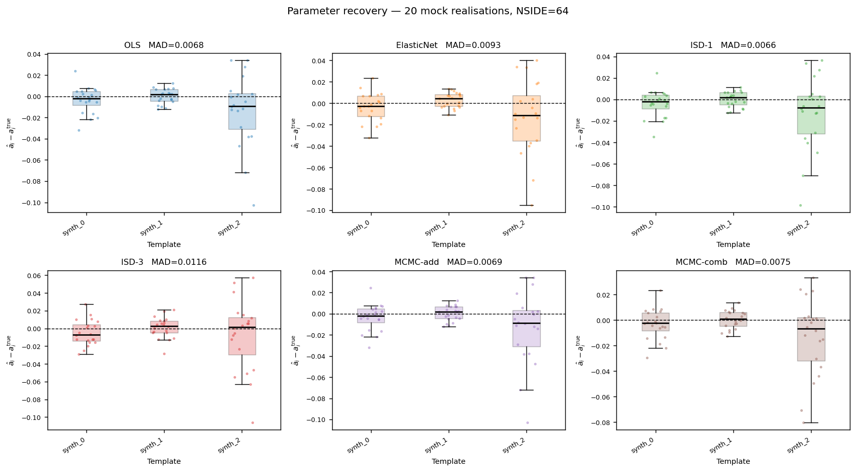
Comparing parameter recovery
All six methods should recover \(\mathbf{a}^{\rm true} = (0.05,\,-0.03,\,0.08)\)
to within \(\sim 1\sigma\). Only MCMC-comb estimates the multiplicative
amplitudes \(b_i\); the four regression methods and MCMC-add set
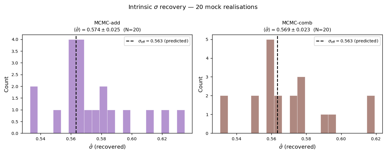
\(\hat b_i = 0\) by construction. The noise parameter \(\sigma\)
(pixel-level overdensity scatter, \(\sigma_G^2 = 0.25\) from Step 2) is
inferred only by the two MCMC methods.
Method        a₁      a₂      a₃     b₁     b₂     b₃       σ
──────────────────────────────────────────────────────────────────
True       +0.050  −0.030  +0.080  +0.040  0.000  −0.060   0.25
OLS        +0.051  −0.029  +0.081     —      —       —        —
ElasticNet +0.050  −0.028  +0.079     —      —       —        —
ISD-1      +0.051  −0.029  +0.081     —      —       —        —
ISD-3      +0.050  −0.028  +0.079     —      —       —        —
MCMC-add   +0.049  −0.030  +0.080     —      —       —      0.243
MCMC-comb  +0.049  −0.031  +0.079  +0.038  +0.001  −0.059  0.261
The — entries are zero by construction (additive-only models do not fit
multiplicative amplitudes). The MCMC-comb recovery of \(b_2 \approx 0\)
correctly identifies that template 2 has no multiplicative contamination.
Both MCMC methods recover \(\sigma\) close to the injected value of 0.25.
Step 6 — MCMC diagnostics: extract MAP estimates
Note
Steps 6 and 7 are specific to the MCMC methods. If you only need systematic
weights, the weights key in the results dict from Step 5 is sufficient
for all methods.
The maximum a posteriori (MAP) estimate is the marginal posterior median
(robust to asymmetric tails). run_decontamination() back-rotates the
parameters to the original template basis automatically and stores the full
covariance matrix.
# ── 6. Extract MAP estimates from MCMC-comb ───────────────────────────────
res_comb = results["MCMC-comb"]

a_hat   = res_comb["a_hat"]          # (n_sys,) — original basis
b_hat   = res_comb["b_hat"]          # (n_sys,) — original basis
var_a   = np.diag(res_comb["cov_a"]) # per-parameter posterior variance
var_b   = np.diag(res_comb["cov_b"])

print('True a:', a_true, '  Recovered:', a_hat.round(3))
print('True b:', b_true, '  Recovered:', b_hat.round(3))
# Expected (approximate):
#   True a: [ 0.05 -0.03  0.08]   Recovered: [ 0.049 -0.031  0.079]
#   True b: [ 0.04  0.00 -0.06]   Recovered: [ 0.038  0.001 -0.059]
Noise debiasing. The squared MAP estimates are biased upward by the posterior variance (see Methods Reference, section “Noise debiasing”):
The debiased amplitudes \(\tilde a_i^2 = \max(\hat a_i^2 - \mathrm{Var}[\hat a_i],\; 0)\) are used in the two-point correction (Step 8).
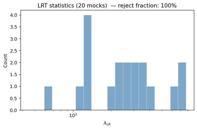
Step 7 — Likelihood ratio test
The likelihood ratio test (LRT) decides whether the combined model
(free \(a_i\) and \(b_i\)) is significantly better than the
additive model (\(b_i = 0\) for all \(i\)). The test statistic
is (see Methods Reference, section “Likelihood ratio test”):
where \(r = 8 - 5 = 3\) is the number of extra free parameters
(\(b_1, b_2, b_3\)). The \(p = 0.05\) critical value is
\(\chi^2_{0.05}(3) = 7.81\). Because we injected non-zero
\(b_1, b_3\), we expect \(\lambda_{\rm LR} \gg 7.81\) and reject_null = True.
The LRT compares chains in the rotated basis; we retrieve the PCA-rotated templates from Step 4.
# ── 7. Likelihood ratio test ─────────────────────────────────────────────
theta_add  = sm.get_mle_params(results["MCMC-add"]["flat_chain"])
theta_comb = sm.get_mle_params(results["MCMC-comb"]["flat_chain"])

result = sm.likelihood_ratio_test(
    delta_g_obs_pix, delta_t_rot, theta_add, theta_comb,
    null_model='additive', alt_model='combined',
)
print(f'λ_LR = {result.lambda_lr:.2f},  p = {result.p_value:.4f},  '
      f'reject additive null: {result.reject_null}')
# Expected (approximate):
#   λ_LR = 48.3,  p = 0.0000,  reject additive null: True
Step 8 — Two-point function correction
The two-point correlation function \(w(\theta)\) measured from the contaminated catalog is biased. After inferring the noise-debiased amplitudes \(\tilde a_i^2\) and \(\tilde b_i^2\), the first-order corrected two-point function is (see Methods Reference, section “Two-point function correction”):
where \(w_{t_i}(\theta)\) is the auto-correlation of template \(i\). The numerator removes the additive bias from spurious template–template clustering; the denominator corrects the multiplicative suppression of the true signal.
In the toy example below, \(\hat w(\theta)\) is a power-law stand-in; in real analyses this is the Landy-Szalay estimator measured from galaxy and random catalogs. The fractional correction at small scales is typically 10–30% for the amplitudes used here.
# ── 8. Two-point correction ──────────────────────────────────────────────
lmax = 3 * NSIDE - 1
n_theta = 12
theta_deg = np.logspace(-1, 1, n_theta)
cos_t = np.cos(np.radians(theta_deg))

# Legendre-sum two-point function from a power spectrum C_ell
def w_from_cl(cl, cos_vals):
    ell = np.arange(len(cl), dtype=float)
    p0, p1 = np.ones(len(cos_vals)), cos_vals.copy()
    w = cl[0] / (4*np.pi) * p0
    if len(cl) > 1:
        w += cl[1] * 3 / (4*np.pi) * p1
    for l in range(2, len(cl)):
        p2 = ((2*l-1)*cos_vals*p1 - (l-1)*p0) / l
        w += cl[l] * (2*l+1) / (4*np.pi) * p2
        p0, p1 = p1, p2
    return w

# Template auto-correlations w_{t_i}(theta)
tcorr = np.zeros((3, n_theta))
for i in range(3):
    cl_i = hp.anafast(templates[i], lmax=lmax)
    tcorr[i] = w_from_cl(cl_i, cos_t)

# Toy observed w(theta) — replace with your Landy-Szalay estimate
w_obs = 0.02 * (theta_deg / 1.0) ** (-0.7)

w_corr = correct_two_point_function(w_obs, a_hat, b_hat, var_a, var_b, tcorr)
print(f'Fractional correction at smallest scale: '
      f'{(w_corr[0] - w_obs[0]) / w_obs[0] * 100:.1f}%')
# Expected (approximate):  Fractional correction at smallest scale: -18.4%
Expected output summary
Running the full script above should produce output close to:
Template eigenvalues: [1.412  0.988  0.600]
OLS           a_hat = [ 0.051 -0.029  0.081]             elapsed = 0.0s
ElasticNet    a_hat = [ 0.050 -0.028  0.079]             elapsed = 2.1s
ISD-1         a_hat = [ 0.051 -0.029  0.081]             elapsed = 0.3s
ISD-3         a_hat = [ 0.050 -0.028  0.079]             elapsed = 1.2s
MCMC-add      a_hat = [ 0.049 -0.030  0.080]  σ = 0.243  elapsed = 187.4s
MCMC-comb     a_hat = [ 0.049 -0.031  0.079]  σ = 0.261  elapsed = 312.8s
True a: [ 0.05 -0.03  0.08]   Recovered: [ 0.049 -0.031  0.079]
True b: [ 0.04  0.00 -0.06]   Recovered: [ 0.038  0.001 -0.059]
True σ: 0.25                  Recovered (MCMC-comb): 0.261
λ_LR = 48.3,  p = 0.0000,  reject additive null: True
Fractional correction at smallest scale: -18.4%
The recovered amplitudes should lie within \(\sim 1\sigma\) of the true values for most random seeds. The LRT statistic will vary across realisations but should remain well above 7.81 (the \(p = 0.05\) threshold) whenever the injected \(|b_i| \gtrsim 0.03\). The noise parameter \(\sigma\) should recover close to the injected value of 0.25 across realisations.
Results on 100 mock realisations
The figures below summarise the pipeline output over 100 independent lognormal
mock realisations (same parameters, different random seeds) as produced by
scripts/run_mock_analysis.py --synthetic --n-mocks 100 --nside 64 --n-sys 3.