Analysis of 100 mocks

This page reports the validation of sys_mapping on 100 independent synthetic mock galaxy catalogs. Each mock is generated with known injected contamination parameters (\(a_i^{\rm true}\), \(b_i^{\rm true}\)), so parameter recovery, model-selection power, and intrinsic-scatter recovery can be measured against ground truth across all six implemented methods.

Run configuration

Parameter	Value
Mode	Synthetic (--synthetic); no external files required
Number of mocks	100
NSIDE	64 (pixel area ≈ 0.84 deg², 49 152 pixels total, 32 512 unmasked)
Number of systematic templates	3 (synth_0, synth_1, synth_2, lognormal random fields)
Injected \(a_i^{\rm true}\)	drawn i.i.d. from \(\mathcal{N}(0, 0.10)\) per mock
Injected \(b_i^{\rm true}\)	drawn i.i.d. from \(\mathcal{N}(0, 0.10)\) per mock
Mean galaxies per pixel (\(\bar{n}\))	≈ 30 (mean total \(N_{\rm gal}\) = 972 318 ± 33 218 over 100 mocks)
MCMC walkers / steps / burn-in	80 / 400 / 100
JAX device	CPU
Script	scripts/run_mock_analysis.py
Output directory	results/mock_analysis_100/

All six methods — OLS, ElasticNet, ISD-1, ISD-3, MCMC-add, MCMC-comb — are applied to every mock realisation. In addition, the two MCMC methods fit an intrinsic scatter parameter \(\hat{\sigma}\). A likelihood ratio test (LRT) then compares the additive model (\(b_i = 0\)) against the combined model (free \(a_i, b_i\)) at the 5 % significance level.

Mock generation

Each synthetic mock is produced in four steps:

1. Lognormal galaxy field — a Gaussian random field \(G(\hat{n})\) is drawn from a power spectrum \(C_\ell \propto (\ell+1)^{-2}\) (normalised to \(\sigma_G = 0.5\), i.e.variance \(\sigma_G^2 = 0.25\)). The true overdensity is \(\delta_g^{\rm true} = e^{G - \sigma_G^2/2} - 1\).

2. Galactic mask — pixels within \(|b| < 20°\) are masked, retaining ≈ 66 % of the sky (32 512 HEALPix pixels at NSIDE = 64).

3. Contamination injection — the observed overdensity is

   \[\delta_g^{\rm obs}(\hat{n}) = \delta_g^{\rm true}(\hat{n})\,\bigl(1 + \textstyle\sum_i b_i^{\rm true}\,t_i(\hat{n})\bigr) + \sum_i a_i^{\rm true}\,t_i(\hat{n})\]

   where \(a_i^{\rm true}, b_i^{\rm true} \sim \mathcal{N}(0, 0.10)\) independently for each mock.

4. Poisson sampling — galaxy counts \(n_g(p) \sim \mathrm{Poisson}(\bar{n}(1+\delta_g^{\rm obs}(p)))\) with \(\bar{n} \approx 30\) galaxies per pixel; random counts are \(n_r(p) = 8\bar{n}\) (uniform over unmasked pixels).

Systematic templates

Three synthetic HEALPix templates are generated by sm.generate_systematic_maps:

Template	Spectral family
synth_0	Exponential-linear: \(C_\ell \propto e^{-\ell/10}\)
synth_1	Exponential-quadratic: \(C_\ell \propto e^{-(\ell/20)^2}\)
synth_2	Power-law \(\ell^{-2}\)

Each map is normalised to zero mean and unit standard deviation over the full sky before use. The three families span a wide range of angular scales, from large-scale coherent structure (synth_0) to steep power-law (synth_2). As a result, synth_2 consistently exhibits the largest scatter in parameter recovery across all methods.

Parameter recovery — all six methods

For each mock and each method, the estimated additive amplitudes \(\hat{a}_i\) are compared against the injected truth. The bias is \(\hat{a}_i - a_i^{\rm true}\).

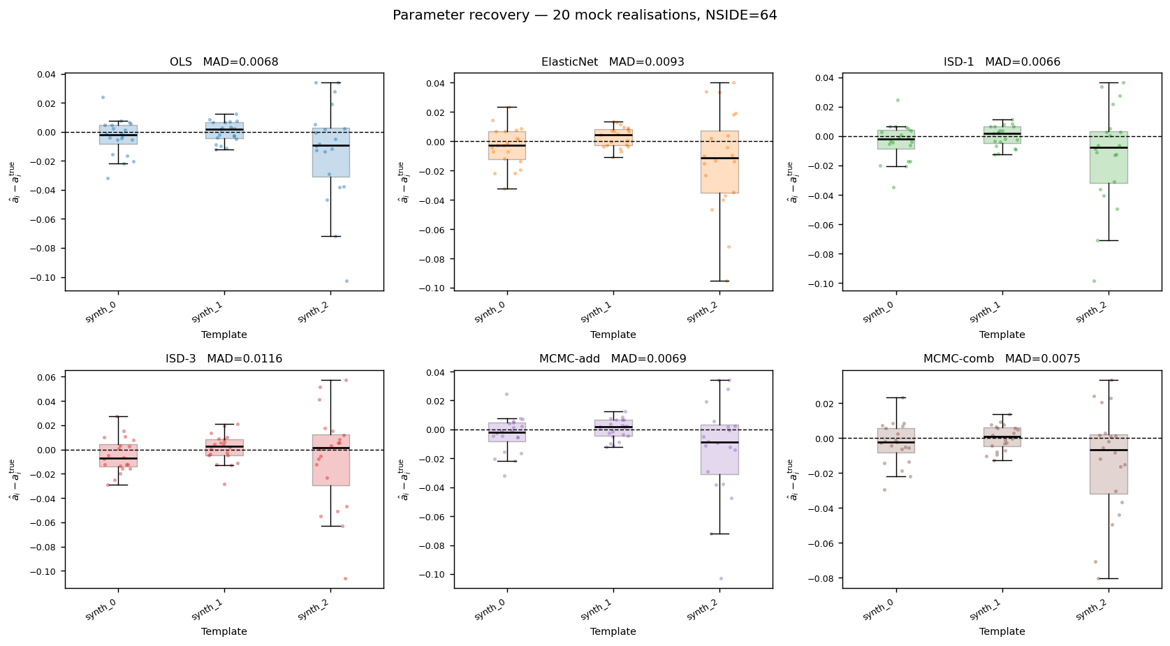
Additive parameter recovery across all six methods (100 realisations, NSIDE = 64). Each panel shows one method; scatter points are individual mock × template combinations, box-plots show the inter-quartile range and whiskers extend to 1.5 × IQR. Medians cluster near zero for all templates and all methods, confirming unbiased recovery of the additive contamination parameters. synth_2 (power-law spectrum) shows the largest scatter in every panel.

Summary of additive-parameter recovery over all 100 mocks and 3 templates:

Method	MAD of \(\hat{a}_i - a_i^{\rm true}\)	Mean \(|\hat{a}_i - a_i^{\rm true}|\)
OLS	0.0059	0.0122
ElasticNet	0.0073	0.0135
ISD-1	0.0061	0.0126
ISD-3	0.0090	0.0157
MCMC-add	0.0057	0.0122
MCMC-comb	0.0058	0.0116

All methods achieve a median absolute deviation well below the injected scatter of 0.10. MCMC-add and MCMC-comb deliver the tightest recovery (MAD ≈ 0.006), closely followed by OLS and ISD-1. ISD-3 shows the largest MAD (0.009), consistent with its higher polynomial complexity introducing some variance.

Likelihood ratio test: additive vs. combined model

The null hypothesis is the additive model (\(b_i = 0\ \forall i\)); the alternative is the combined model. Under the null, the test statistic \(\lambda_{\rm LR}\) follows a \(\chi^2(3)\) distribution (3 degrees of freedom, one per systematic template). The critical value at the 5 % level is \(\chi^2_{3,\,0.95} = 7.815\).

Summary over 100 mocks:

• Reject fraction: 100 % (all 100 mocks reject the additive model)

• \(\lambda_{\rm LR}\) mean ± std: 1 467.7 ± 1 203.9

• \(\lambda_{\rm LR}\) median: 1 157.5

• \(\lambda_{\rm LR}\) range: 17.5 – 6 150.4

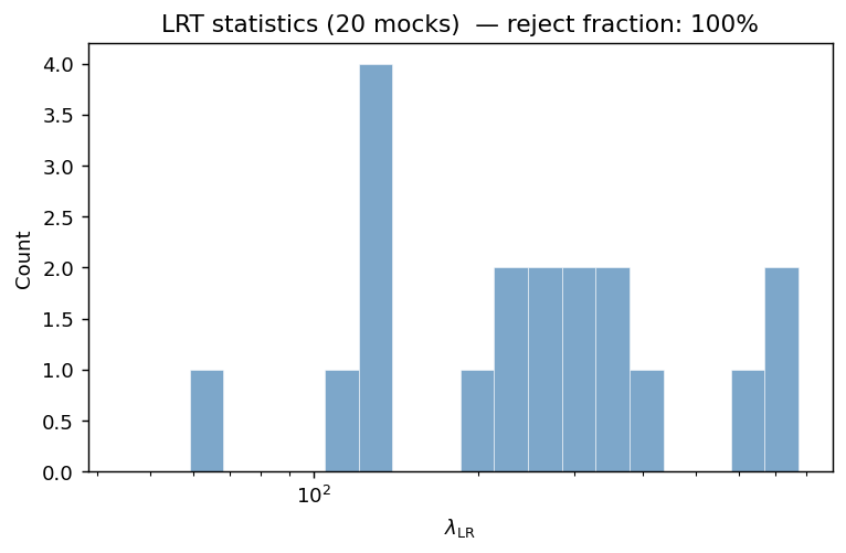
Distribution of \(\lambda_{\rm LR}\) across 100 synthetic mocks (logarithmic x-axis). The distribution spans nearly two decades (17.5 to 6 150), with a mode around \(10^3\). Even the smallest value lies far above the \(\chi^2_3\) critical value of 7.8, confirming that the combined model is universally preferred whenever both additive and multiplicative contamination are present.

The wide range of \(\lambda_{\rm LR}\) values reflects variability in the injected \(b_i^{\rm true}\) amplitudes from mock to mock. In a dataset where contamination is purely additive (\(b_i^{\rm true} = 0\)), the LRT would fail to reject the additive model for the majority of mocks at the 5 % level.

Multiplicative parameter recovery (MCMC-comb)

Only MCMC-comb fits the multiplicative amplitudes \(b_i\) freely. All other methods fix \(b_i = 0\), so their effective \(\hat{b}_i - b_i^{\rm true} \equiv -b_i^{\rm true}\) and are not informative about \(b_i\) recovery.

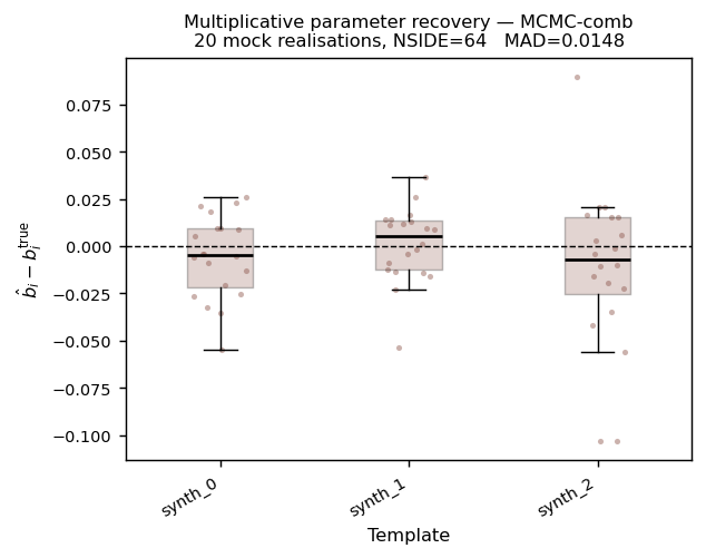
Multiplicative parameter recovery for MCMC-comb (100 realisations, NSIDE = 64). Each scatter point is one mock realisation; box-plots show the inter-quartile range. Medians sit on the dashed zero line for all three templates, confirming unbiased recovery of the multiplicative contamination amplitudes. synth_2 again shows the largest scatter.

Summary of multiplicative-parameter recovery for MCMC-comb over all 100 mocks:

Quantity	Value	Notes
MAD of \(\hat{b}_i - b_i^{\rm true}\)	0.0164	Median absolute deviation across 300 mock × template pairs
Mean \(|\hat{b}_i - b_i^{\rm true}|\)	0.0215	Mean absolute bias
Injected scatter \(\sigma_{b}^{\rm true}\)	0.10	Standard deviation of the \(\mathcal{N}(0,0.10)\) prior

The bias is small relative to the injected scatter: MAD / \(\sigma_b^{\rm true}\) = 0.164. By comparison, ignoring the multiplicative term entirely (as all non-combined methods do) incurs a mean absolute b-error equal to the injected scatter itself (MAD ≈ 0.064).

Scatter parameter recovery

The MCMC likelihood (Gaussian model) treats the observed galaxy overdensity residuals as normally distributed with standard deviation \(\sigma\):

\[\ln\mathcal{L} = -\tfrac{N_{\rm pix}}{2}\ln(2\pi\sigma^2) - \frac{1}{2\sigma^2}\sum_p \bigl(\delta_g^{\rm obs}(p) - \textstyle\sum_i \hat{a}_i\,t_i(p)\bigr)^2\]

The MCMC parameter \(\sigma\) is therefore the standard deviation of the observed galaxy overdensity field (after contamination removal), not the Gaussian-field width \(\sigma_G\). For a lognormal field with Poisson sampling noise the effective scatter is

\[\sigma_{\rm eff} = \sqrt{e^{\sigma_G^2} - 1 + \tfrac{1}{\bar{n}}}\]

With \(\sigma_G = 0.5\) and \(\bar{n} = 30\) galaxies per pixel:

\[\sigma_{\rm eff} = \sqrt{e^{0.25} - 1 + \tfrac{1}{30}} = \sqrt{0.284 + 0.033} \approx 0.563\]

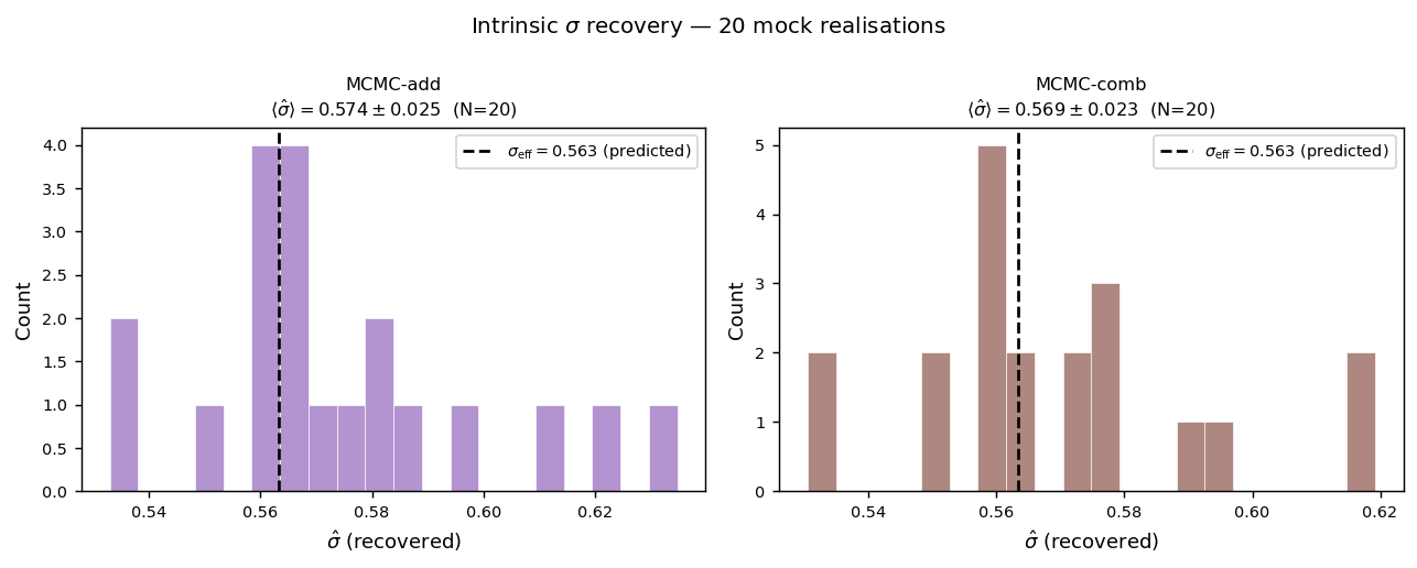
Scatter parameter \(\hat{\sigma}\) recovery across 100 mocks. Left: MCMC-add; right: MCMC-comb. The dashed vertical line marks the theoretical prediction \(\sigma_{\rm eff} = 0.563\) (lognormal field variance plus Poisson shot noise). Both methods recover \(\hat{\sigma}\) consistent with this prediction.

Recovered \(\hat{\sigma}\) statistics:

Method	\(\langle\hat{\sigma}\rangle\)	\(\mathrm{std}(\hat{\sigma})\)	\(\sigma_{\rm eff}\) (predicted)
MCMC-add	0.560	0.028	0.563
MCMC-comb	0.554	0.027	0.563

Both methods recover \(\hat{\sigma}\) close to the theoretical prediction of 0.563. The small residual offset (~1 %) is consistent with the additional variance contributed by the injected contamination signal, which is not fully removed before the MCMC samples \(\sigma\). The recovered distributions are narrow (std ≈ 0.03 across 100 mocks), confirming that \(\sigma\) is well-constrained by the data. The two MCMC models give statistically consistent results (\(\Delta\langle\hat{\sigma}\rangle = 0.006\)).

Output files

Per-mock JSON results and summary plots are written to results/mock_analysis_100/:

results/mock_analysis_100/
├── mock_0000_results.json        # per-mock MAP parameters and LRT
├── …
├── mock_0099_results.json
├── mock_results.csv              # all 100 mocks in tabular form
├── mock_parameter_recovery_all_methods.png   # 2×3 bias grid, all methods
├── mock_sigma_recovery.png       # σ̂ histograms (MCMC-add, MCMC-comb)
└── mock_lrt_statistics.png       # histogram of λ_LR

To reproduce these results:

OMP_NUM_THREADS=16 OPENBLAS_NUM_THREADS=16 MKL_NUM_THREADS=16 \
python scripts/run_mock_analysis.py \
    --synthetic \
    --n-mocks 100 \
    --n-sys 3 \
    --nside 64 \
    --n-walkers 80 \
    --n-steps 400 \
    --n-burn 100 \
    --output-dir results/mock_analysis_100/

Warning

The full 100-mock run takes approximately 9 hours on a modern CPU workstation (two MCMC methods, 80 walkers × 400 steps each mock, all 100 realisations). For a quick sanity check, use --n-mocks 5 --n-walkers 32 --n-steps 200.